8  Causal inference with G-computation

Randomized experiments are often considered to be the “gold standard” research design for causal inference. Assigning individuals to different treatments at random ensures that, on average and under ideal conditions, the groups we compare have similar background characteristics. This overall similarity gives us more confidence that any differences to emerge between groups are caused by the treatments of interest. Randomized experiments are powerful tools but, unfortunately, they are often impractical or unethical. In such cases, we must turn to observational data.

Drawing causal inference from observational data can be difficult. Often, factors beyond the analyst’s control influence both the exposure to treatment and the outcome of interest. Such confounding variables can introduce bias in our estimates of the treatment effect.

Imagine a study designed to assess the impact of daily vitamin D supplementation (treatment) on bone density (outcome). If the analyst finds that individuals taking vitamin D have higher bone density, they may be tempted to conclude that supplementation directly enhances bone health. However, people who choose to take vitamin D might also be more health-conscious and engage in other bone-strengthening activities, such as regular exercise or consuming a calcium-rich diet. These confounding factors can obscure the true causal effect of vitamin D supplements on bone density. They can introduce bias in our estimates.

G-computation¹ is a method developed to draw causal inference from observational data. The idea is simple. First, we fit a statistical model that controls for confounders. Then, we use the fitted model to “predict” or “impute” what would happen to an individual under alternative treatment scenarios. Finally, we compare counterfactual predictions to derive an estimate of the treatment effect (Hernán and Robins 2020).

As we will see below, G-computation estimates are equivalent to the counterfactual predictions and comparisons discussed in Chapters 5 and 6. They are also closely related to the estimates we can obtain by Inverse Probability Weighting (IPW), another popular causal inference tool. IPW and G-computation impose similar identification assumptions, with one key difference: the former requires us to model the process that determines who gets treated, whereas the latter requires us to model the outcome variable.²

The next section introduces the key estimands that analysts can target via G-computation: the average treatment effect (ATE), average treatment effect on the treated (ATT), and average treatment effect on the untreated (ATU). Subsequent sections present the estimation procedure as a sequence of three steps: model, impute, and compare.

8.1 Estimands: ATE, ATT, ATU

Our goal is to estimate the effect of a treatment \(D\) on an outcome \(Y\). To express this effect as a formal estimand, and to understand the assumptions required to target that estimand, we need to introduce a bit of notation from the potential outcomes tradition of causal inference (Section 1.1.3, Imbens and Rubin (2015), Morgan and Winship (2015)).

The first term we need to define represents the value of the treatment, or explanatory variable. When \(D_i=1\), the individual \(i\) is assigned to the treatment group. When \(D_i=0\), \(i\) is part of the control group.

The second term represents the outcome variable. Here, it is essential to draw a distinction between the actual value of the outcome, and its potential values. The actual outcome is what we observe for individual \(i\) in our dataset: \(Y_i\). In contrast, the potential outcomes are written with superscripts: \(Y_i^0\) and \(Y_i^1\). They represent the outcomes that would occur in counterfactual worlds where \(i\) receives different treatments. \(Y_i^0\) is the value of the outcome in a hypothetical world where \(i\) belongs to the control group. \(Y_i^1\) is the value of the outcome in a hypothetical world where \(i\) belongs to the treatment group. Crucially, only one potential outcome can ever be observed at any given time, for any given individual. Since \(i\) cannot be part of both the treatment and control groups simultaneously, we can never measure the values of both \(Y_i^1\) and \(Y_i^0\).

The ambitious analyst would love to estimate the Individual Treatment Effect (ITE), defined as the difference between outcomes for \(i\) under different treatment regimes: \(Y_i^1-Y_i^0\). Unfortunately, since we can only observe one of the two potential outcomes, the ITE is impossible to compute. This is what some have called the fundamental problem of causal inference.

To circumvent this problem, we turn away from individual-level estimands, and consider three aggregated quantities of interest: ATE, ATT, and ATU. These three quantities are related, but they invite different interpretations and impose different assumptions (Greifer and Stuart 2021).

\[\begin{align*} E[Y_i^1 - Y_i^0] && \mbox{(ATE)} \\ E[Y_i^1 - Y_i^0|D_i=1] && \mbox{(ATT)} \\ E[Y_i^1 - Y_i^0|D_i=0] && \mbox{(ATU)} \end{align*}\]

8.1.1 Interpretation

The ATE estimates the average effect of the treatment on the outcome in the entire study population. The ATE helps us answer this question: Should a program or treatment be implemented universally?

The ATT estimates the average effect of the treatment on the outcome in the subset of study participants who actually received it. The ATT helps us answer this question: Should a program or treatment be withheld from the people currently receiving it?

The ATU estimates the average effect of the treatment on the subgroup of participants who did not, in fact, get it. The ATU helps us answer this question: Should a program or treatment be extended to those who did not initially receive it?

8.1.2 Assumptions

Estimating the ATE, ATT, or ATU requires us to accept four assumptions, with varying levels of stringency (Greifer and Stuart 2021; Chatton and Rohrer 2024).

First, conditional exchangeability or no unmeasured confounding. This assumption states that potential outcomes must be independent of treatment assignment, conditional on a set of control variables (\(Z_i\)). More formally, we can write this assumption as: \(Y_i^1,Y_i^0 \perp D_i \mid Z_i\).

Imagine a person who considers entering a training program (\(D_i\)) designed to improve their likelihood of finding a job (\(Y_i\)). If that person has good reasons to believe they will be employed, regardless of whether they enroll in the program or not (\(Y_i^1=Y_i^0\)), they are unlikely to sign up. Similarly, imagine a doctor who recommends a certain medication (\(D_i\)) only to the patients who are most likely to benefit from it (\(Y_i^1>Y_i^0\)). In both cases, potential outcomes are linked to the treatment assignment mechanism: \(D_i \not\perp Y_i^1,Y_i^0\). In both cases, the conditional exchangeability assumption is violated, unless the analyst can control for all relevant confounders.

When estimating the ATE, conditional exchangeability must hold across the entire population. When estimating the ATT, however, this stringent assumption can be relaxed somewhat. The intuition is straightforward: since the ATT is computed solely based on units in the treatment group, we can observe all instances of the \(Y_i^1\) potential outcomes. Thus, to estimate the ATT, we only need to make assumptions about the unobserved \(Y_i^0\) potential outcomes; we only need to adjust for confounders that link treatment assignment to participants’ outcomes under the control condition. Analogously, estimating the ATU only requires conditional exchangeability to hold in the treatment condition.

Second, positivity. This assumption requires study participants to have a non-zero probability of belonging to each treatment arm: \(0<P(D_i=1\mid Z_i)<1\). In practice, this condition can be violated for a number of reasons, such as when certain individuals fail to meet eligibility criteria to receive a certain treatment.

When we estimate the ATE, positivity must hold across the entire sample. However, when we estimate the ATT, the positivity assumption can be relaxed somewhat: \(P(D_i=1|Z_i)<1\). This new condition means that no participant can be certain to receive the treatment, but that some participants can be ruled ineligible. Analogously, we can estimate the ATU by accepting a weaker form of positivity, where every participant must have some chance to be treated: \(P(D_i=1|Z_i)>0\).

Third, consistency.³ This assumption requires the intervention to be well-defined; there must be no ambiguity about what constitutes “treatment” and “control.” For example, in a medical study, consistency may require that all participants in the treatment group be administered the same drug, under the same conditions, with the same dosage. In the context of a job training intervention, consistency might require strict adherence to a specific program design, with fixed hours of in-person teaching, number of assignments, internship requirements, etc.

Fourth, non-interference. This final assumption says that potential outcomes for one participant should not be affected by the treatment assignments of other individuals. Assigning one person (or group) to a treatment regime cannot lead to contagion or generate externalities for other participants in the study.

When these four assumptions hold, we can estimate the effect of a treatment via G-computation. The remainder of this chapter describes this estimation strategy in three steps: model, impute, and compare.

8.2 Model

To illustrate how to estimate the ATE, ATT, and ATU using G-computation, let’s consider the study by Imbens, Rubin, and Sacerdote (2001): Estimating the Effect of Unearned Income on Labor Earnings, Savings, and Consumption: Evidence from a Survey of Lottery Players. In that article, the authors conducted a survey to estimate the effect of winning large lottery prizes on economic behavior. They studied a range of behaviors and outcomes, for different subgroups of the population. In this chapter, we focus on estimating the effect of winning a big lottery prize on labor earnings in subsequent years.

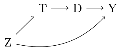
The “treatment” is a binary variable equal to one if an individual won a lottery prize, and zero otherwise (\(D\)). The outcome of interest is the average labor earnings over the next six years (\(Y\)). Winning lottery numbers are chosen randomly, but the probability that any given person wins a prize is not purely random: it depends on how many tickets that individual purchased (\(T\)). Finally, we know that socio-demographic characteristics (\(Z\)) like age, education, and employment status, can influence both the number of tickets that a person buys and their labor earnings. These causal relationships are illustrated in the graph below.

Imbens, Rubin, and Sacerdote (2001) collected survey responses to measure the variables in this graph. Their dataset includes a variety of information about 437 respondents, including 194 who won small lottery prizes, and 43 who won big prizes. For simplicity, we will only compare individuals who won a big prize to those who won nothing at all.

library(marginaleffects)
dat <- get_dataset("lottery")
dat <- subset(dat, win_big == 1 | win == 0)

head(dat, n = 2)

# A data frame: 2 × 26
    age college education   man prize tickets   win win_big win_small  work
* <dbl>   <dbl>     <dbl> <dbl> <dbl>   <dbl> <dbl>   <dbl>     <dbl> <dbl>
1    76       0        12     0     0       2     0       0         0     0
2    59       1        16     1     0       2     0       0         0     1
# ℹ 16 more variables: year <dbl>, earnings_pre_avg <dbl>,
#   earnings_post_avg <dbl>, earnings_pre_1 <dbl>, earnings_pre_2 <dbl>,
#   earnings_pre_3 <dbl>, earnings_pre_4 <dbl>, earnings_pre_5 <dbl>,
#   earnings_pre_6 <dbl>, earnings_post_1 <dbl>, earnings_post_2 <dbl>,
#   earnings_post_3 <dbl>, earnings_post_4 <dbl>, earnings_post_5 <dbl>,
#   earnings_post_6 <dbl>, earnings_post_7 <dbl>

The first G-computation step is to define an outcome equation, that is, to specify a parametric regression model for the dependent variable. The primary goal of this regression model is to control for confounders, that is, to ensure that we meet the conditional exchangeability assumption stated in Section 8.1.2.

As noted above, the process that determines which lottery tickets are winning is purely random, but the probability that any given individual wins depends on the number of tickets they bought. This means that the treatment assignment (\(D\)) is not completely independent from the potential outcomes (\(Y_i^1,Y_i^0\)). To satisfy the conditional exchangeability assumption,⁴ our statistical model must control for the number of tickets (\(T\)) that each survey respondents bought and/or for all the \(S\) covariates that link \(D\) to \(Y\).

This regression model can be simple or flexible. It can be purely linear, or include a non-linear link function, multiplicative interactions, polynomials, or splines (see Chapter 10). The model can satisfy the conditional exchangeability assumption using a minimal set of control variables (\(T\)), or it can include a more covariates (\(S\)) to improve precision (see Section 9.1 on regression adjustement).

Here, we fit a linear regression where the treatment variable (win_big) is interacted with the number of tickets bought (tickets) and a series of demographic characteristics, including gender, age, employment, and pre-lottery labor earnings. To interact treatment and covariates, we insert a star * symbol and parentheses in the regression formula.

mod <- lm(
  earnings_post_avg ~ win_big * (
    tickets + man + work + age + education + college + year +
    earnings_pre_1 + earnings_pre_2 + earnings_pre_3),
  data = dat)

summary(mod)

                         Estimate Std. Error t value Pr(>|t|)
(Intercept)            1302.25641 1099.91390   1.184   0.2374
win_big                1327.56843 2435.94389   0.545   0.5862
tickets                   0.13340    0.31632   0.422   0.6736
man                      -0.85082    1.27346  -0.668   0.5046
work                      3.24753    1.61780   2.007   0.0457
age                      -0.23762    0.05330  -4.459   <0.001
education                -0.53448    0.53047  -1.008   0.3145
college                   3.03770    2.08575   1.456   0.1464
year                     -0.64566    0.55434  -1.165   0.2451
earnings_pre_1            0.05247    0.16390   0.320   0.7491
earnings_pre_2           -0.04408    0.18013  -0.245   0.8069
earnings_pre_3            0.86314    0.10288   8.390   <0.001
win_big:tickets          -0.17277    0.54143  -0.319   0.7499
win_big:man               1.51214    4.38811   0.345   0.7307
win_big:work             -0.73710    5.23892  -0.141   0.8882
win_big:age               0.13777    0.14432   0.955   0.3406
win_big:education         0.61646    1.11628   0.552   0.5812
win_big:college           9.62742    5.50191   1.750   0.0812
win_big:year             -0.67657    1.22789  -0.551   0.5821
win_big:earnings_pre_1   -0.23283    0.41698  -0.558   0.5770
win_big:earnings_pre_2   -0.26659    0.49941  -0.534   0.5939
win_big:earnings_pre_3   -0.12319    0.27092  -0.455   0.6497

8.3 Impute

The second G-computation step is to impute—or predict—the outcome for each observed individual, under different hypothetical treatment regimes. To do this, we create two identical copies of the dataset used to fit the model, and we use the transform function to fix the win_big variable to counterfactual values.

# counterfactual dataset with all participants in the control group
d0 <- transform(dat, win_big = 0)

# counterfactual dataset with all participants in the treatment group
d1 <- transform(dat, win_big = 1)

Using these two datasets, we predict the expected earnings_post_avg for each participant under counterfactual treatment regimes.

# expected outcomes if all participants belonged to the control group
p0 <- predictions(mod, newdata = d0)

# expected outcomes if all participants belonged to the treatment group
p1 <- predictions(mod, newdata = d1)

To take stock of what we have done so far, we can inspect the original dataset, and compare the predicted outcomes for an arbitrary survey respondent: the person in the sixth row of our dataset. By subsetting the data frame, we see that this person did not, in fact, win a big lottery prize.

dat[6, "win_big"]

[1] 0

Using our fitted model, we predicted that this person’s average labor earnings—without lottery winnings—would be:

p0[6, "estimate"]

[1] 31.91696

If this individual belonged to the treatment group instead (win_big=1), our model would predict lower earnings:

p1[6, "estimate"]

[1] 24.5759

Thus, our model expects that, for an individual with these socio-demographic characteristics, winning the lottery is likely to decrease labor earnings. In the next section, we compare these predicted outcomes more systematically, at the aggregate level, to estimate the ATE, ATT, and ATU.

8.4 Compare

To estimate the treatment effect of win_big via G-computation, we aggregate individual-level predictions from the two counterfactual worlds. We can do this by extracting the vectors of estimates computed above, and by calling the mean() function.

The average predicted outcome in the control counterfactual is:

mean(p0$estimate)

[1] 17.42834

The average predicted outcome in the treatment counterfactual is:

mean(p1$estimate)

[1] 11.86662

A more convenient way to obtain the same quantities is to call the avg_predictions() function from the marginaleffects package. As noted in Chapter 5, using the variables argument computes predicted values on a counterfactual grid, and the by argument marginalizes with respect to the focal variable. The results are the same as those we computed “manually,” but they come with standard errors and confidence intervals.

avg_predictions(mod,
  variables = "win_big",
  by = "win_big")

win_big	Estimate	Std. Error	z	Pr(>|z|)	2.5 %	97.5 %
0	17.4283	0.570125	30.56933	< 0.001	16.31092	18.5458
1	11.8666	2.278477	5.20814	< 0.001	7.40089	16.3324

The ATE is the difference between the two estimates printed above. We can compute it by subtraction, or using the avg_comparisons() function.

avg_comparisons(mod,
  variables = "win_big",
  newdata = dat)

Estimate	Std. Error	z	Pr(>|z|)	2.5 %	97.5 %
-5.56172	2.34872	-2.36798	0.0178856	-10.1651	-0.958313

This last value is the G-computation estimate of the average treatment effect of win_big on earnings_post_avg. On average, our model estimates that moving from the loser to the winner group increases the predicted outcome by -5.6.

To compute the ATT, we use the same approach as above, but restrict our attention to the subset of individuals who were actually treated. We use the subset() function to select rows of the original dataset with treated individuals, and feed the resulting grid to the newdata argument.

avg_comparisons(mod, 
  variables = "win_big", 
  newdata = subset(dat, win_big == 1))

Estimate	Std. Error	z	Pr(>|z|)	2.5 %	97.5 %
-9.48789	1.82431	-5.2008	< 0.001	-13.0635	-5.9123

The ATU is computed analogously, by restricting our attention to the subset of untreated individuals.

avg_comparisons(mod, 
  variables = "win_big", 
  newdata = subset(dat, win_big == 0))

Estimate	Std. Error	z	Pr(>|z|)	2.5 %	97.5 %
-4.90989	2.59001	-1.8957	0.0579996	-9.98622	0.166441

It is interesting to notice that the ATE, ATT, and ATU are substantially different from one another. This finding underscores the importance of clearly defining the quantity of interest before estimating and interpreting statistical models (Section 1.2).

8.5 Additional considerations

TODO:

• Benefits: Beyond the obvious benefits (simplicity and uncertainty quantification), using marginaleffects gives analysts access to all the features described in previous chapters: complex hypothesis or equivalence tests; subgroup analyses; robust or clustered standard errors; easy bootstrap and simulation based inference; etc.
• Uncertainty
  • Conditional variance: Dowd, Greene, and Norton (2014) Qu and Luo (2015)
  • Unconditional variance: Hansen and Overgaard (2024)
  • Bootstrap Hernán and Robins (2020)

Chatton, Arthur, and Julia M. Rohrer. 2024. “The Causal Cookbook: Recipes for Propensity Scores, g-Computation, and Doubly Robust Standardization.” Advances in Methods and Practices in Psychological Science 7 (1): 25152459241236149. https://doi.org/10.1177/25152459241236149.

Dowd, Bea E., William H. Greene, and Edward C. Norton. 2014. “Computation of Standard Errors.” Health Services Research 49 (2): 731–50.

Greifer, Noah, and Elizabeth A Stuart. 2021. “Choosing the Estimand When Matching or Weighting in Observational Studies.” arXiv e-Prints, arXiv–2106.

Hansen, S. N., and M. Overgaard. 2024. “Variance Estimation for Average Treatment Effects Estimated by g-Computation.” Metrika. https://doi.org/10.1007/s00184-024-00962-4.

Hernán, Miguel A, and James M Robins. 2020. Causal Inference: What If. Boca Raton: Chapman & Hall/CRC.

Imbens, Guido W, and Donald B Rubin. 2015. Causal Inference in Statistics, Social, and Biomedical Sciences. Cambridge university press.

Imbens, Guido W, Donald B Rubin, and Bruce I Sacerdote. 2001. “Estimating the Effect of Unearned Income on Labor Earnings, Savings, and Consumption: Evidence from a Survey of Lottery Players.” American Economic Review 91 (4): 778–94.

Morgan, Stephen L, and Christopher Winship. 2015. Counterfactuals and Causal Inference. Cambridge University Press.

Pearl, Judea. 2009. Causality. Cambridge university press.

Qu, Y., and J. Luo. 2015. “Estimation of Group Means When Adjusting for Covariates in Generalized Linear Models.” Pharmaceutical Statistics 14 (1): 56–62. https://doi.org/10.1002/pst.1741.

---

1. The estimation procedure described in this chapter is sometimes referred to as the “Parametric G-Formula.”

2. G-computation and IPW can be combined to create a “doubly-robust” estimator with useful properties. A comprehensive presentation of IPW and doubly-robust estimation lies outside the scope of this book. Interested readers can refer to the marginaleffects.com website for tutorials, and to Chatton and Rohrer (2024) for intuition and comparisons.

3. Formally, if \(D_i=1\) then \(Y_i=Y_i^1\), and if \(D_i=0\) then \(Y_i=Y_i^0\). The consistency and non-interference assumptions are often stated together under the label “Stable Unit Treatment Value Assumption”, or SUTVA.

4. In the Pearl (2009) tradition, we would say: “to satisfy the backdoor criterion.”