Survival analysis is concerned with analyzing the (causal) effects of one or more variables on a time-to-event outcome, such as time until death or time until the occurrence of a disease. One of the main issues of survival analysis in practice is that the time-to-event outcomes are often right-censored, meaning that it is only known that the event of interest did not occur up until some point in time for some individuals. The most popular class of models that directly deals with right-censoring are Cox proportional hazards models (Cox 1972). Although very useful, these models are not marginal models. They only produce hazard ratios (HR), which are conditional quantities. As such, they do not directly estimate practically relevant causal estimands by themselves (Hernán 2010). This makes the parameter estimates produced by such models quite difficult to interpret in practical settings, an issue that is shared by a majority of other time-to-event models as well.
To interpret results from survival models, authors have recommended reporting marginal estimands, such as the difference or ratio between counterfactual survival probabilities (Klein et al. 2007; Royston and Parmar 2013; Uno et al. 2014). These counterfactual probabilities may also be presented visually as “adjusted survival curves,” allowing for easier presentation of the results (Denz et al. 2023). A popular and statistically efficient way to calculate these quantities is the use of g-computation (Robins 1986).
The marginaleffects package is uniquely suited to perform these tasks. It allows users to compute a wide array of intuitive and meaningful quantities of interest, and to compare them to one another. The package also allows users to easily specify complex hypothesis tests, to study interactions or effect modification.
Crucially, the syntax and approach used to interpret survival models is exactly the same as for any of the 100+ model types supported by marginaleffects. Users who have read the (free) Model to Meaning will feel right at home.
This vignette illustrates how to use marginaleffects to estimate various marginal causal estimands in survival analysis on the basis of time-to-event models. Our goal is mainly to give a non-technical overview of the capabilities of the package. For more technical and detailed explanations of the shown material we recommend consulting standard textbooks on survival analysis.
32.1 Example Data and Model
Let’s consider a classic real-data example from the survival analysis literature: the rotterdam dataset from the survival R package (Hofman et al. 1991). The rotterdam dataset, obtained from the Rotterdam tumor bank, contains information on 2982 breast cancer patients. It includes variables related to patient demographics, clinical characteristics, and survival outcomes. The dataset is used in survival analysis to study the relationship between predictors and survival time.
For the purposes of this vignette, we will try to analyze the causal effect of a hormonal treatment on the time until death. In the rotterdam dataset, the hormonal treatment is a binary variable called hormon, where 0 indicates no treatment and 1 means that the patient did receive a treatment. The time until death is coded as a classic time-to-event variable with two columns: dtime and death. Here, dtime is the time until death or right-censoring in days and deathis the event status indicator, where 0 indicates that the patient was still alive at dtime and 1 indicates that the patient died at dtime. The study did not randomize the hormon treatment, meaning that we have to adjust for confounding as is usual in observational data.
For the analysis of the data we will first fit a standard Cox proportional hazards model with the time to death or right-censoring as the response variable and the hormonal treatment as independent variable. Additionally, we will include grade, which is an ordinal variable reflecting the level of tumor differentiation, and age at surgery, a continuous variable indicating the age in years as further independent variables. To account for a possible non-linear relationship between age and the time until death we model this variable using a natural spline with two degrees of freedom, as shown below:
model<-coxph(Surv(dtime, death)~hormon+grade+ns(age, df =2), data =rotterdam)summary(model)
From the summary() output alone it looks like the hormonal treatment leads to a faster time until death on average with a HR of ~ 1.34, even after adjustment for age and grade. We will investigate this further below.
Warning
This notebook reports uncertainty estimates obtained via non-parametric bootstrapping, using the vcov="rsample" argument. This is important because the default standard errors in marginaleffects may be severely anti-conservative. See the section on “Uncertainty” below for an important note on this topic.
Replicate the entire dataset once for each combination of hormon and dtime that we wish to consider.
Compute the predicted survival probability for every row in this grid.
Take the average of the predicted survival probabilities for each combination of hormon and dtime.
The function we use to implement these steps is avg_predictions(). We set type="survival" to obtain the average counterfactual predictions on the survival probability scale. Other options would be to use type="risk" to obtain the predictions on a death probability scale instead.
The by argument indicates that we want to marginalize survival probabilities over each unique combination of hormon and dtime.
The vcov argument is set to "rsample" to use non-parametric bootstrapping to compute the standard errors, implemented by the rsample package.
Because we want to calculate counterfactual predictions, we also had to define the newdata argument using a call to the datagrid() function. As usual, this argument controls over which values of the predictors the predictions should be made. Since there are many dtime values, replicating the full dataset would be very memory- and computationally-intensive. Therefore, we specify a grid with 25 equally spaced points in time between the first and the last occurring event time. Then, we feed the grid to the avg_predictions() function.
nd<-datagrid( hormon =0:1, dtime =seq(36, 7043, length.out =25), grid_type ="counterfactual", model =model)p<-avg_predictions(model, type ="survival", by =c("dtime", "hormon"), vcov ="rsample", newdata =nd)tail(p)
The Estimate column shows the estimated average “counterfactual” survival probability at dtime for hormon = 0 and hormon = 1. These can be interpreted as:
the fraction of individuals that we would expect to survive, on average, up to dtime, if every individual in the population had or had not received hormonal treatment.
Consider this subset of estimates, where dtime is at its maximum value:
The first row suggests that if we had not intervened on any individual in the dataset, our model expects that about 27% percent of individuals would still be alive by dtime=7043. In contrast, the second row suggests that if we had intervened on every individual in the dataset, our model expects that only about 18% percent of individuals would still be alive by dtime=7043.
Warning
This counterfactual interpretation of the estimated average survival probabilities only holds if the model is correctly specified, and if four fundamental causal identification assumptions hold:
positivity
counterfactual consistency
no-interference
conditional exchangeability
These assumptions are described in detail in Hernán and Robins (2020) and many other books and articles on causal inference based methods.
32.2.1 Plot
Since the output of avg_predictions() is a data frame, we can use it directly to plot the results, using ggplot2, base R, or any other plotting package. Here, we use the tinyplot package to display the adjusted survival curves:
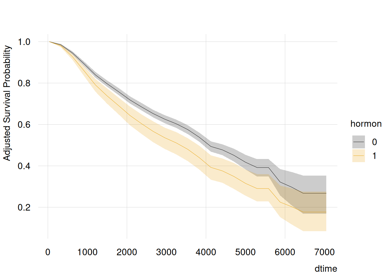
with(p, {tinyplot( x =dtime, y =estimate, ymin =conf.low, ymax =conf.high, by =hormon, type ="ribbon", ylab ="Adjusted Survival Probability")})
The resulting plot shows the survival curves for both treatment options of hormon, adjusted for age and grade. As can be seen quite clearly from the plot alone, the confidence intervals do not overlap for the majority of the shown time, but not all points in time. Using only the HR from the model, we would have been unable to make such distinctions or plot this graphic.
32.2.2 Hypothesis Testing
The plot in the previous section showed a difference between the two hormon groups at almost every point in time. The confidence intervals did not overlap much, which could lead the analyst to believe that the difference between survival probabilities in the treatment and control groups are distinguishable. In some situations, however, it might be necessary to formally compare the survival probabilities at a specific point in time using a statistical hypothesis test (Klein et al. 2007). In other words, one may wish to check if we can reject this null hypothesis:
At time \(t\), the difference between the estimated survival probability for patients in group hormon=1 and hormon=0 is equal to zero.
This kind of null hypothesis can be tested easily with the avg_predictions() function. In the code below, we specify a new grid with three different vales of dtime: 1000, 4000, and 7000. Then, we use the convenient formula syntax of the hypothesis argument to compute differences in estimated survival probabilities for each dtime.
nd<-datagrid( hormon =0:1, dtime =c(1000, 4000, 7000), grid_type ="counterfactual", model =model)p<-avg_predictions(model, hypothesis =difference~reference|dtime, type ="survival", by =c("dtime", "hormon"), vcov ="rsample", newdata =nd)p
Note that the syntax is essentially identical to the syntax used when estimating the adjusted survival curves, with the only difference being that we focus on three points in time in the datagrid() call, and that we additionally specified the hypothesis argument.
The Estimate column of the output now includes the estimated difference between counterfactual survival probabilities at \(t\in\{1000,4000,7000\}\). For all three time points, the difference in expected survival probabilities for the two hormon groups is negative, and the confidence intervals exclude zero. This means that, for all three time points, we can reject the null hypothesis that the survival probabilities are equal for patients receiving hormonal treatment and those not receiving it.
Another option would be to use the ratio of the two survival probabilities instead. To do this, we only change the left-hand side of the hypothesis formula.
p<-avg_predictions(model, hypothesis =ratio~reference|dtime, type ="survival", by =c("dtime", "hormon"), vcov ="rsample", newdata =nd)p
Here, the Estimate argument shows the ratio of the two survival probabilities at \(t\) instead of the difference, again with associated 95% confidence interval. The three intervals exclude 1, which means we can reject the null hypothesis that estimated survival is identical in both hormon groups.
As noted in the hypothesis testing chapter, users may define much more complicated hypotheses or equivalence tests, to compare subgroups and look into interactions or treatment effect heterogeneity.
32.2.3 Interactions and heterogeneous treatment effects
In the real world, we often encounter heterogeneous treatment effects, meaning that the causal effect of one variable on an outcome is not necessarily the same in different groups of individuals. For example, we might be interested in assessing whether the effect of the hormonal treatment differs by values of grade. The classic approach to assess such heterogeneity is to allow a multiplicative interactions in the Cox model formula:
Although there is nothing inherently wrong with this approach, the results from the Cox model alone are not easy to interpret. In this case the HR of hormon no longer refers to the HR of the hormonal treatment in general, but only to the HR of hormonin the grade = 2 group, which can be confusing. Additionally, the HRs only show conditional, not marginal, effects. Using g-computation we can instead visualize adjusted survival curves for hormon by grade and perform additional hypothesis tests.
Even though the model and the estimand changed, the syntax required to estimate the counterfactual survival probabilities stays essentially the same. The only change we have to perform is that we have to add grade to the datagrid() call and to the by argument. To make the output a little more comprehensible we focus three points in time: \(t\in\{1000, 4000, 7000\}\).
nd<-datagrid( hormon =unique, grade =unique, dtime =c(1000, 4000, 7000), grid_type ="counterfactual", model =model)p<-avg_predictions(model, type ="survival", by =c("dtime", "hormon", "grade"), vcov ="rsample", newdata =nd)p
The output now contains twelve rows, one for each combination of dtime, hormon and grade. For example, the first row shows the estimated average survival probability at \(t=1000\) would be 91%, in a counterfactual world where every patient has hormon=0 and grade = 2.
Now, imagine we want to test a complex hypothesis such as:
What is the difference in expected (counterfactual) survival probabilities between two specific types of individuals?
Row 1: hormon=1 and grade=2 and dtime=1000
Row 7: hormon=0 and grade=2 and dtime=4000
We could first compute the estimated differences manually as:
We can of course plot counterfactual predictions for different subgroups. Here, we consider 25 equally spaced points in time, with 4 different combinations of hormon and grade.
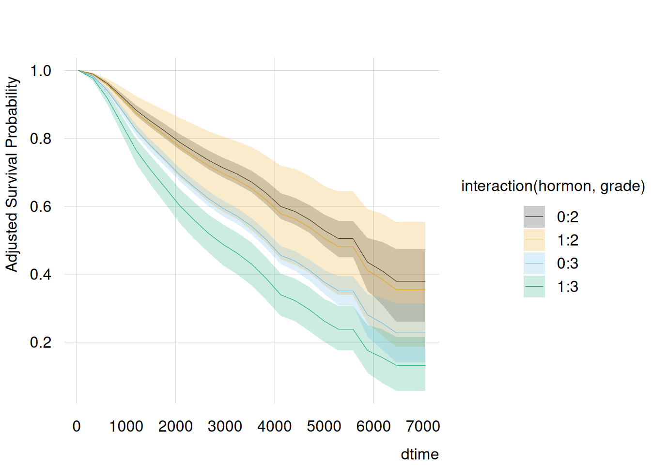
nd<-datagrid( hormon =unique, grade =unique, dtime =seq(36, 7043, length.out =25), grid_type ="counterfactual", model =model)p<-predictions(model, type ="survival", by =c("dtime", "hormon", "grade"), vcov ="rsample", newdata =nd)with(p, {tinyplot(estimate~dtime|hormon+grade, ymin =conf.low, ymax =conf.high, type ="ribbon", ylab ="Adjusted Survival Probability")})
Instead of one adjusted survival curve per hormon group, we now get four adjusted survival curves in total. In the resulting graph we get some indication of an interaction effect between grade and hormon. For grade = 2 the curves of hormon = 0 and hormon = 1 are very similar, whereas they do seem to be somewhat further apart for grade = 3. It is, however, difficult to make a solid judgement here because the confidence intervals of all groups are quite wide and mostly overlapping.
32.3 Counterfactual comparisons
So far, we have focused on the average counterfactual predictions (on the survival scale) for different combinations of predictors. The marginaleffects package also allows us to take a more explicitly “interventional” approach, focused on the estimation of treatment effects. Indeed, the Counterfactual Comparisons chapter explains how to use the comparisons() and avg_comparisons() functions to answer a series of key questions.
To start, we ask: What is the estimated average treatment effect of hormon on the survival probability of people in our sample, at time \(t=5000\).
nd<-datagrid( dtime =5000, grid_type ="counterfactual", model =model)cmp<-avg_comparisons(model, variables ="hormon", type ="survival", vcov ="rsample", newdata =nd)cmp
For individuals in grade = 2, moving from hormon = 0 to hormon = 1 is associated with a -2 percentage point change in the expected survival probability at \(t=5000\). For individuals in grade = 3, the corresponding change is -11 percentage points.
At first glance, these two estimates seem different. Are they really? To test this formally, we add the hypothesis argument to the previous call.
cmp<-avg_comparisons(model, hypothesis =difference~reference, variables ="hormon", type ="survival", by ="grade", vcov ="rsample", newdata =nd)cmp
The difference in estimated survival probabilities between hormon = 0 and hormon = 1 is different for different values of grade. However, the confidence interval on the difference (in differences) covers zero. This means that we cannot reject the null hypothesis that the effect of hormon on survival is identical for people with grade=2 and those with grade=3.
As explained elsewhere in the package documentation, the hypothesis argument allows very flexible input types. For example, we could identify estimates by row number and specify hypothesis tests like hypothesis = "b1 - b2 = 0" or hypothesis = "b1 / b2 = 1". Alternatively, we could supply custom functions or formulas to test even more complicated hypotheses about heterogeneity.
32.4 Uncertainty
Before concluding, it is useful to briefly discuss the challenge of estimating uncertainty around marginal estimates in the types of models considered here. One important challenge arises because the log-likelihood of the Cox proportional‐hazards model naturally factorizes into a partial component that involves only the regression coefficients and a baseline component that involves the cumulative hazard.
\[
h(t\mid x)=h_{0}(t)\,\exp\{x^{\top}\beta\},
\]
with baseline hazard \(h_{0}(t)\) and coefficients \(\beta\).
The key innovation that underpins this model is that we do not need to optimize the likelihood of the full model. Instead, if we are willing to accept some assumptions (i.e., proportional hazards), we can proceed with the partial likelihood.
Once we fit the model in this way, we can compute predictions on the linear-predictor scale easily.
The variance of those predictions can be obtained via the delta method, through the estimated variance–covariance matrix of the coefficients alone. Unfortunately, other quantities of interest are functions of more than just the estimated coefficients. For functions that depend on the baseline hazard (e.g., survival or cumulative hazard curves) a second source of variability enters through the estimation of \(H_{0}(t)\).
marginaleffects applies the multivariate delta method to propagate uncertainty from \(\hat\beta\) to any user‑defined function \(g(\hat\beta)\). For Cox models the current implementation ignores the extra variability in \(\hat H_{0}(t)\). When effect estimates depend on the baseline this omission produces anti‑conservative confidence intervals—often by a non‑trivial margin.
A simple remedy is the non‑parametric bootstrap: resample subjects (or clusters) with replacement, refit the Cox model in each replicate, and re‑calculate the target function. Because every replicate re‑estimates both \(\beta\)and\(H_{0}(t)\), the resulting empirical distribution captures their joint variability without analytic derivations. While computationally heavier, this method usually restores nominal coverage and works seamlessly with marginaleffects via the vcov = "rsample" argument or the inferences() function.
32.5 Conclusion
This vignette has shown that the marginaleffects can be used to easily compute very useful marginal estimands, that greatly facilitate the interpretation of survival models. For users who are already familiar with the marginaleffects package this is particularly easy, because the syntax required for survival analysis is exactly the same syntax that can be used for non-survival models. Additionally, the included capabilities to test complex hypotheses dealing with interaction and effect modification is, to the best of our knowledge, not implemented elsewhere.
Note, however, that although g-computation is one of the most popular and most efficient methods to estimate the causal estimands described here, it is not the only method and may not always be the best choice (Denz et al. 2023). Due to its’ sole reliance on a time-to-event model, the resulting estimates are very susceptible to model misspecification. Other methods, such as augmented inverse probability of treatment weighting (Wang 2018) or targeted maximum likelihood estimation (Cai and Laan 2020), additionally use a model for the treatment assignment process and are doubly-robust in the sense that only one of the models needs to be correctly specified to obtain unbiased estimates. Additionally, we recommend that users keep in mind that the causal interpretation of the produced estimates of any method are only valid given the causal identifiability assumptions, which do not always hold in practice.
32.6 Thanks
The marginaleffects authors gratefully acknowledge Robin Denz for writing the first version of this vignette.
Cai, Weixin, and Mark J. van der Laan. 2020. “One-Step Targeted Maximum Likelihood Estimation for Time-to-Event Outcomes.”Biometrics 76: 722–33. https://doi.org/10.1111/biom.13172.
Denz, Robin, Renate Klaaßen-Mielke, and Nina Timmesfeld. 2023. “A Comparison of Different Methods to Adjust Survival Curves for Confounders.”Statistics in Medicine 42 (10): 1461–79. https://doi.org/10.1002/sim.9681.
Hernán, Miguel A., and James M. Robins. 2020. Causal Inference: What If. CRC Press.
Hofman, A., D. E. Grobbee, P. T. de Jong, and F. A. van den Ouweland. 1991. “Determinants of Disease and Disability in the Elderly: The Rotterdam Elderly Study.”European Journal of Epidemiology 7 (4): 403–22. https://doi.org/10.1007/BF00145007.
Klein, John P., Brent Logan, Mette Harhoff, and Per Kragh Andersen. 2007. “Analyzing Survival Curves at a Fixed Point in Time.”Statistics in Medicine 26: 4505–19. https://doi.org/10.1002/sim.2864.
Robins, James. 1986. “A New Approach to Causal Inference in Mortality Studies with a Sustained Exposure Period: Application to Control of the Healthy Worker Survivor Effect.”Mathematical Modeling 7: 1393–512.
Royston, Patrick, and Mahesh K. B. Parmar. 2013. “Restricted Mean Survival Time: An Alternative to the Hazard Ratio for the Design and Analysis of Randomized Trials with a Time-to-Event Outcome.”BMC Medical Research Methodology 13 (152). https://doi.org/10.1186/1471-2288-13-152.
Uno, Hajime, Brian Claggett, Lu Tian, et al. 2014. “Moving Beyond the Hazard Ratio in Quantifying the Between-Group Difference in Survival Analysis.”Journal of Clinical Oncology 32 (22): 2380–85. https://doi.org/10.1200/JCO.2014.55.2208.
Wang, Jixian. 2018. “A Simple, Doubly Robust, Efficient Estimator for Survival Functions Using Pseudo Observations.”Pharmaceutical Statistics 17: 38–48. https://doi.org/10.1002/pst.1834.