library(marginaleffects)
mod <- glm(am ~ wt + drat, family = binomial, data = mtcars)
mfx <- avg_slopes(mod)
tab <- print(mfx, "tinytable")
class(tab)
#> [1] "tinytable"
#> attr(,"package")
#> [1] "tinytable"45 Tables
45.1 tinytable
By default, marginaleffects will print results to the console. However, it is easy to print in many other formats using the tinytable package, which supports a variety of output formats, including HTML, LaTeX, markdown, Word, and Typst.
https://vincentarelbundock.github.io/tinytable/
For example,
We can then style this table using tinytable’s style_tt() function, add grouping columns or rows with group_tt(), format the content with format_tt(), etc. We can also save the table to file using save_tt(). For instance, to save to a Word document:
save_tt(tab, "/path/to/table.docx")
45.2 modelsummary
We can summarize the results of the comparisons() or slopes() functions using the modelsummary package.
library(modelsummary)
library(marginaleffects)

mod <- glm(am ~ wt + drat, family = binomial, data = mtcars)
mfx <- avg_slopes(mod)

modelsummary(mfx)| (1) | |
|---|---|
| drat | 0.278 |
| (0.168) | |
| wt | -0.217 |
| (0.080) | |
| Num.Obs. | 32 |
| AIC | 22.0 |
| BIC | 26.4 |
| Log.Lik. | -8.011 |
| F | 3.430 |
| RMSE | 0.28 |
The same results can be visualized with modelplot():
modelplot(mfx)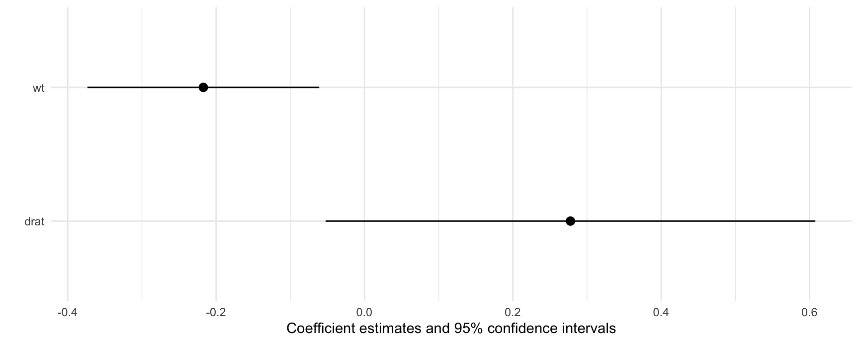
When using the avg_comparisons() function (or the avg_slopes() function with categorical variables), the output will include two columns to uniquely identify the quantities of interest: term and contrast.
dat <- mtcars
dat$gear <- as.factor(dat$gear)
mod <- glm(vs ~ gear + mpg, data = dat, family = binomial)

cmp <- avg_comparisons(mod)
get_estimates(cmp)
#> # A tibble: 3 × 9
#>   term  contrast estimate std.error statistic    p.value s.value conf.low conf.high
#>   <chr> <chr>       <dbl>     <dbl>     <dbl>      <dbl>   <dbl>    <dbl>     <dbl>
#> 1 gear  4 - 3      0.0372    0.137      0.272 0.785        0.348  -0.230     0.305
#> 2 gear  5 - 3     -0.340     0.0988    -3.44  0.000588    10.7    -0.533    -0.146
#> 3 mpg   +1         0.0609    0.0128     4.78  0.00000178  19.1     0.0359    0.0859
We can use the shape argument of the modelsummary function to structure the table properly:
modelsummary(cmp, shape = term + contrast ~ model)| (1) | ||
|---|---|---|
| gear | 4 - 3 | 0.037 |
| (0.137) | ||
| 5 - 3 | -0.340 | |
| (0.099) | ||
| mpg | +1 | 0.061 |
| (0.013) | ||
| Num.Obs. | 32 | |
| AIC | 26.2 | |
| BIC | 32.1 | |
| Log.Lik. | -9.101 | |
| F | 2.389 | |
| RMSE | 0.31 |
Cross-contrasts can be a bit trickier, since there are multiple simultaneous groups. Consider this example:
mod <- lm(mpg ~ factor(cyl) + factor(gear), data = mtcars)
cmp <- avg_comparisons(
  mod,
  variables = c("gear", "cyl"),
  cross = TRUE)
get_estimates(cmp)
#> # A tibble: 4 × 10
#>   term  contrast_cyl contrast_gear estimate std.error statistic p.value s.value conf.low conf.high
#>   <chr> <chr>        <chr>            <dbl>     <dbl>     <dbl>   <dbl>   <dbl>    <dbl>     <dbl>
#> 1 cross 6 - 4        4 - 3            -5.33      2.77     -1.93 0.0542     4.21    -10.8  0.0953
#> 2 cross 6 - 4        5 - 3            -5.16      2.63     -1.96 0.0500     4.32    -10.3  0.000165
#> 3 cross 8 - 4        4 - 3            -9.22      3.62     -2.55 0.0108     6.53    -16.3 -2.13
#> 4 cross 8 - 4        5 - 3            -9.04      3.19     -2.84 0.00453    7.79    -15.3 -2.80
As we can see above, there are two relevant grouping columns: contrast_gear and contrast_cyl. We can simply plug those names in the shape argument:
modelsummary(
  cmp,
shape = contrast_gear + contrast_cyl ~ model)| gear | cyl | (1) |
|---|---|---|
| 4 - 3 | 6 - 4 | -5.332 |
| (2.769) | ||
| 8 - 4 | -9.218 | |
| (3.618) | ||
| 5 - 3 | 6 - 4 | -5.156 |
| (2.631) | ||
| 8 - 4 | -9.042 | |
| (3.185) | ||
| Num.Obs. | 32 | |
| R2 | 0.740 | |
| R2 Adj. | 0.701 | |
| AIC | 173.7 | |
| BIC | 182.5 | |
| Log.Lik. | -80.838 | |
| F | 19.190 | |
| RMSE | 3.03 |