23 Heterogeneity
This short vignette illustrates how to use recursive partitioning to explore treatment effect heterogeneity. This exercise inspired by Scholbeck et al. 2022.
As pointed out in other vignettes, most of the quantities estimated by the marginaleffects package are “conditional”, in the sense that they vary based on the values of all the predictors in our model. For instance, consider a Poisson regression that models the number of hourly bike rentals in Washington, DC:
We can use the comparisons() function to estimate how the predicted outcome changes for a 5 celsius increase in temperature:
cmp <- comparisons(mod, variables = list(temp = 5))
cmp
 Estimate Std. Error    z Pr(>|z|)    S 2.5 % 97.5 %
      423       55.3 7.65   <0.001 45.5   315    531
      384       51.8 7.40   <0.001 42.7   282    485
      320       40.1 8.00   <0.001 49.5   242    399
      360       43.4 8.29   <0.001 52.9   275    445
      370       45.7 8.10   <0.001 50.7   281    460
--- 721 rows omitted. See ?print.marginaleffects ---
      418       48.3 8.66   <0.001 57.6   323    513
      426       50.0 8.51   <0.001 55.7   328    524
      366       44.0 8.33   <0.001 53.5   280    453
      304       40.6 7.50   <0.001 43.9   225    384
      343       40.5 8.47   <0.001 55.2   264    422
Term: temp
Type: response
Comparison: +5
The output printed above includes 727 rows: 1 for each of the rows in the original bikes dataset. Indeed, since the “effect” of a 5 unit increase depends on the values of covariates, different unit of observation will typically be associated with different contrasts.
In such cases, a common strategy is to compute an average difference, as described in the G-Computation vignette:
avg_comparisons(mod, variables = list(temp = 5))
 Estimate Std. Error    z Pr(>|z|)    S 2.5 % 97.5 %
      689       64.1 10.7   <0.001 87.1   564    815

Term: temp
Type: response
Comparison: +5
Alternatively, one may be interested in exploring heterogeneity in effect sizes in different subsets of the data. A convenient way to achieve this is to use the ctree function of the partykit package. This function allows us to use recursive partitioning (conditional inference trees) to find subspaces with reasonably homogenous estimates, and to report useful graphical and textual summaries.
Imagine that we are particularly interested in how the effect of temperature on bike rentals varies based on day of the week and season:
tree <- ctree(
    estimate ~ weekday + season,
    data = cmp,
    control = ctree_control(maxdepth = 2)
)
Now we can use the plot() function to draw the distributions of estimates for the effect of an increase of 5C on bike rentals, by week day and season:
plot(tree)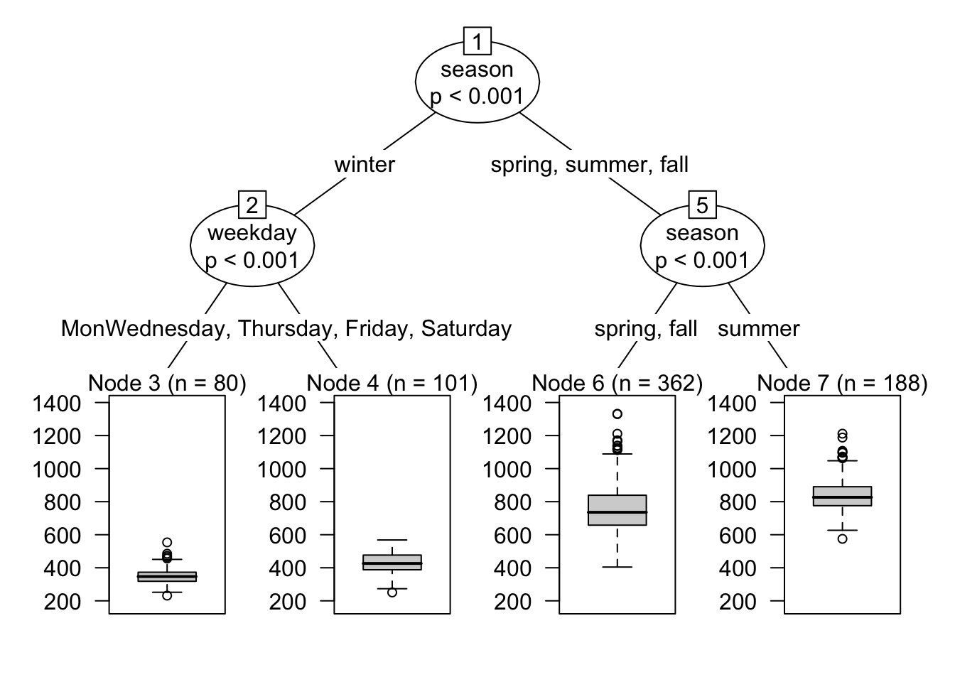
To obtain conditional average estimates for each subspace, we first use the predict() function in order to place each observation in the dataset in its corresponding “bucket” or “node”. Then, we use the by argument to indicate that comparisons() should compute average estimates for each of the nodes in the tree:
dat <- transform(bikes, nodeid = predict(tree, type = "node"))
comparisons(mod,
    variables = list(temp = 5),
    newdata = dat,
    by = "nodeid")
 nodeid Estimate Std. Error     z Pr(>|z|)    S 2.5 % 97.5 %
      3      352       37.2  9.46   <0.001 68.1   279    425
      4      433       42.9 10.08   <0.001 76.9   348    517
      6      757       70.4 10.74   <0.001 87.0   619    895
      7      841       80.9 10.40   <0.001 81.8   683   1000

Term: temp
Type: response
Comparison: +5
The four nodeid values correspond to the terminal nodes in this tree:
print(tree)
Model formula:
estimate ~ weekday + season

Fitted party:
[1] root
|   [2] season in winter
|   |   [3] weekday in Monday, Tuesday, Sunday: 351.902 (n = 80, err = 248952.3)
|   |   [4] weekday in Wednesday, Thursday, Friday, Saturday: 432.617 (n = 101, err = 461053.1)
|   [5] season in spring, summer, fall
|   |   [6] season in spring, fall: 756.522 (n = 362, err = 7548395.3)
|   |   [7] season in summer: 841.324 (n = 188, err = 2116175.9)

Number of inner nodes:    3
Number of terminal nodes: 4