19 Bootstrap
This vignette demonstrates how to use bootstrap methods for inference with the marginaleffects package.
19.1 Parallelization
The bootstrap is an incredibly powerful and flexible method to quantify the uncertainty around estimates. Unfortunately, it can be quite computationally expensive. In some cases, parallelization can significantly speed up the process. This is most beneficial when bootstrap sample size (R) is large (≥ 1000); model fitting is computationally expensive; you have multiple CPU cores available.
Under the hood, marginaleffects uses the future framework to enable parallel processing. This requires calling the plan() function, and specifying a couple global options:
-
marginaleffects_parallel_inferences: Set toTRUEto enable parallel processing -
marginaleffects_parallel_packages: Character vector of package names used to fit the model.
19.2 Simple example
All the objects produced by the marginaleffects can be passed to the inferences() function to compute bootstrap confidence intervals. For example, fit a simple model to the iris dataset and compute average comparisons.
mod <- lm(Sepal.Length ~ Sepal.Width + Species, data = iris)
avg_comparisons(mod)
        Term            Contrast Estimate Std. Error     z Pr(>|z|)     S 2.5 % 97.5 %
 Sepal.Width +1                     0.804      0.106  7.56   <0.001  44.5 0.595   1.01
 Species     versicolor - setosa    1.459      0.112 13.01   <0.001 126.2 1.239   1.68
 Species     virginica - setosa     1.947      0.100 19.47   <0.001 277.9 1.751   2.14

Type: response
The default confidence intervals reported above were computed using the delta method. We can obtain bootstrap-based estimates by piping the command into inferences():
avg_comparisons(mod) |> inferences(method = "rsample")
        Term            Contrast Estimate 2.5 % 97.5 %
 Sepal.Width +1                     0.804 0.602   1.03
 Species     versicolor - setosa    1.459 1.255   1.67
 Species     virginica - setosa     1.947 1.770   2.13

Type: response
This also works with other marginaleffects functions:
avg_predictions(mod, by = "Species") |> inferences(method = "rsample")
    Species Estimate 2.5 % 97.5 %
 setosa         5.01  4.94   5.08
 versicolor     5.94  5.80   6.06
 virginica      6.59  6.44   6.73

Type: responsehypotheses(mod, hypothesis = ratio ~ sequential) |> inferences(method = "rsample")
                               Hypothesis Estimate 2.5 % 97.5 %
 (Sepal.Width) / ((Intercept))               0.357 0.201  0.646
 (Speciesversicolor) / (Sepal.Width)         1.815 1.528  2.308
 (Speciesvirginica) / (Speciesversicolor)    1.335 1.183  1.540
The inferences() function supports multiple bootstrap methods, and includes arguments to control some aspects of the procedure, including R to determine the number of resamples. Additional (undocumented) arguments will be passed to the underlying bootstrap function, such as rsample::bootstraps(). This allows users to supply arguments such as strata or pool. See ?rsample::bootstraps for details.
19.3 Custom Estimation Procedures
Sometimes analysts need to use the bootstrap to compute uncertainy around more complex estimation procedures that go beyond the standard marginal effects workflow. For example, one may want to proceed in three steps:
- Fit a logistic regression model to the treatment in order to estimate propensity scores.
- Fit a linear model to the outcome using the estimated propensity scores as weights.
- Compute the average treatment effect using G-computation and weights with the
avg_comparisons()function.
The bootstrap allows us to take into account the uncertainty in all stages of estimation. This can be useful in a variety of other scenarios, such as complex survey designs, or machine learning applications where analysts wish to bootstrap the entire ML pipeline.
To implement a custom estimation procedure, we define an estimator argument in inferences() function. estimator() must
- Take a data frame as input
- Return an object of class
hypotheses,predictions,slopes, orcomparisons
19.3.1 Example: Bootstrap with Propensity Score Weighting
library(marginaleffects)

lalonde <- get_dataset("lalonde")

# Define custom estimator function
# input: data frame
# output: marginaleffects object
estimator <- function(data) {
    # Step 1: Estimate propensity scores
    fit1 <- glm(treat ~ age + educ + race, family = binomial, data = data)
    ps <- predict(fit1, type = "response")

    # Step 2: Fit weighted outcome model
    m <- lm(re78 ~ treat * (re75 + age + educ + race),
        data = data, weight = ps
    )

    # Step 3: Compute average treatment effect by G-computation
    avg_comparisons(m, variables = "treat", wts = ps, vcov = FALSE)
}

# Test the estimator on the full dataset
estimator(lalonde)
Estimate
1146
Term: treat
Type: response
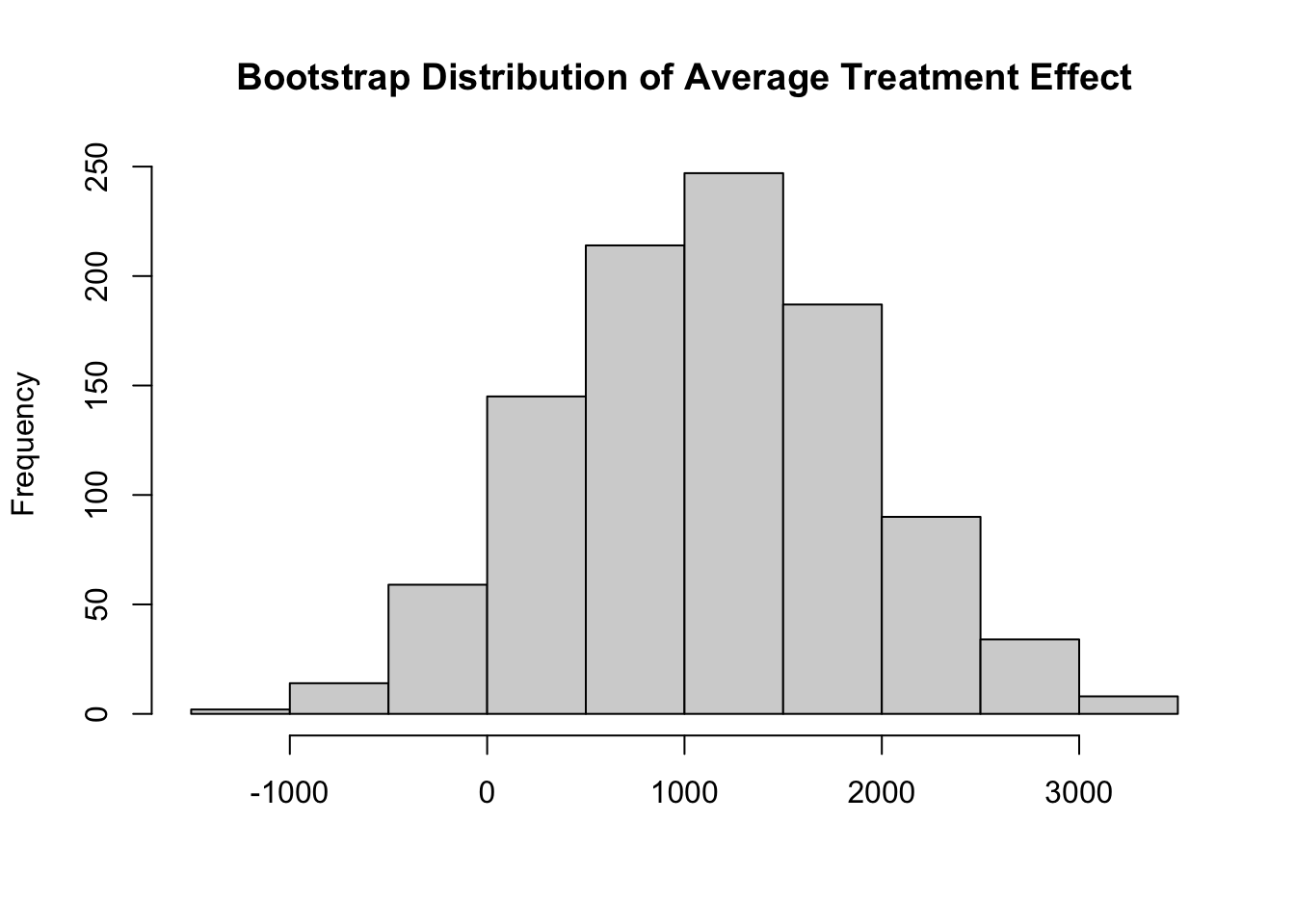
Comparison: 1 - 0# Bootstrap the entire procedure
cmp <- inferences(lalonde, method = "rsample", estimator = estimator)The benefit of this approach is that it abstracts away from the mechanics of bootstrapping. We do not need to interact with the rsample or boot packages directly. We do not need to post-process or reshape the draws to obtain the format of interest. Indeed, the output is a standard marginaleffects object, that can be manipulated with all the standard tools, and comes with a nice pretty-print method:
cmp
 Estimate 2.5 % 97.5 %
     1146  -390   2672

Term: treat
Type: response
Comparison: 1 - 0
It also allows us to examine the bootstrap distribution easily, by extracting draws in a variety of convenient format using the get_draws() helper function from marginaleffects.
19.3.2 Estimator function with arguments
The estimator argument only accepts a single function, and we cannot pass additional arguments to that function. However, we can use a function factory to create a custom estimator that accepts additional arguments.
estimator_factory <- function(outcome = "Sepal.Width", predictor = "Sepal.Length") {
  estimator_function <- function(data) {
    f <- as.formula(sprintf("%s ~ %s * factor(Species)", outcome, predictor))
    mod <- lm(f, data = data)
    avg_slopes(mod, variables = predictor, by = "Species")
  }
}

fun <- estimator_factory(outcome = "Petal.Width", predictor = "Sepal.Length")
inferences(iris, estimator = fun, method = "rsample", R = 100)
    Species Estimate  2.5 % 97.5 %
 setosa       0.0831 0.0196  0.153
 versicolor   0.2094 0.1366  0.281
 virginica    0.1214 0.0269  0.196

Term: Sepal.Length
Type: response
Comparison: dY/dX
fun <- estimator_factory(outcome = "Petal.Width", predictor = "Petal.Length")
inferences(iris, estimator = fun, method = "rsample", R = 100)
    Species Estimate  2.5 % 97.5 %
 setosa        0.201 0.0641  0.396
 versicolor    0.331 0.2597  0.417
 virginica     0.160 0.0906  0.283

Term: Petal.Length
Type: response
Comparison: dY/dX