The concepts and post-estimation tools introduced in earlier chapters—predictions, counterfactual comparisons, and slopes—are largely model-agnostic; they are applicable to both statistical and machine learning approaches. These tools are especially effective for model description, a task that is very important in machine learning applications, where analysts need to audit and understand how models respond to different inputs.1
Auditing and describing machine learning models is essential to ensure that predictions remain fair, and that they are driven by factors compatible with the substantive knowledge of domain experts. For instance, in credit scoring systems, evaluating how variations in applicant characteristics—such as income, employment status, or ethnicity—influence creditworthiness assessments helps detect and mitigate potential biases. Similarly, in hiring algorithms, how models weight different candidate attributes—like education level or years of experience—can help recruiters use models in decision-making. Audits and model description are crucial to improve the transparency and interpretability of data analyses.
13.1tidymodels and mlr3
The marginaleffects package facilitates model description and auditing by allowing analysts to compute and visualize predictions, counterfactual comparisons, and slopes. It integrates seamlessly with some of the most prominent machine learning frameworks in R (tidymodels and mlr3) and Python (Scikit Learn).
tidymodels is a collection of packages in R designed for modeling and machine learning using tidyverse principles, offering a cohesive interface for data preprocessing, modeling, and validation (Kuhn and Wickham 2020). mlr3 is a modern, object-oriented framework in R that provides a comprehensive suite of tools for machine learning, including a wide array of algorithms, resampling methods, and performance measures (Lang et al. 2019). By supporting both tidymodels and mlr3, marginaleffects enables users to interpret a wide variety of machine learning models . Scikit Learn is a powerful Python library for machine learning that provides simple and efficient tools for data mining and data analysis (Pedregosa et al. 2011).
A comprehensive introduction to machine learning in general, or to particular frameworks, lies outside the scope of this book.2 Instead, this chapter shows a very simple example to demonstrate that the workflow built-up in previous chapters applies in straightforward fashion to this new context.
Let us consider data on Airbnb rental properties in London, collected and distributed by Békés and Kézdi (2021). This dataset includes information on over 50,000 units, including features such as the unit type (single room or entire unit), number of bedrooms, parking, or internet access. The primary outcome of our analysis is the rental price of each unit.
To begin, we load the tidymodels and marginaleffects libraries, read the data, and display the first rows and columns.
The airbnb dataset includes 55 columns and 52717 rows. We split those rows into a training set to fit the model, and a test set to make predictions and evaluate the model’s behavior.
The next block of code holds the core tidymodels fitting commands. The boost_tree() function specifies the model type. In this case, we use the XGBoost implementation of boosted trees, to predict a continuous outcome (i.e., “regression”). Users who prefer a different prediction algorithm could swap this line for linear_reg(), rand_forest(), bart(), etc. The recipe() function identifies the outcome variable (price), and initiates a data pre-processing “recipe,” that is, a series of steps to transform the raw data into a suitable format for model fitting. step_dummy() is used to convert categorical predictors into dummy variables. Finally, the workflow() function combines the model and the pre-processing recipe, and the fit() function fits the model to the training data.
With the fitted model in hand, we now use the predictions() function to generate predictions in the test set. As usual, predictions() returns a simple data frame with the quantity of interest in the estimate column, and the original data in separate columns. Thus, we can easily check the quality of our predictions in the test set by plotting the predicted values of the outcome (estimate) against the actually observed values (price).
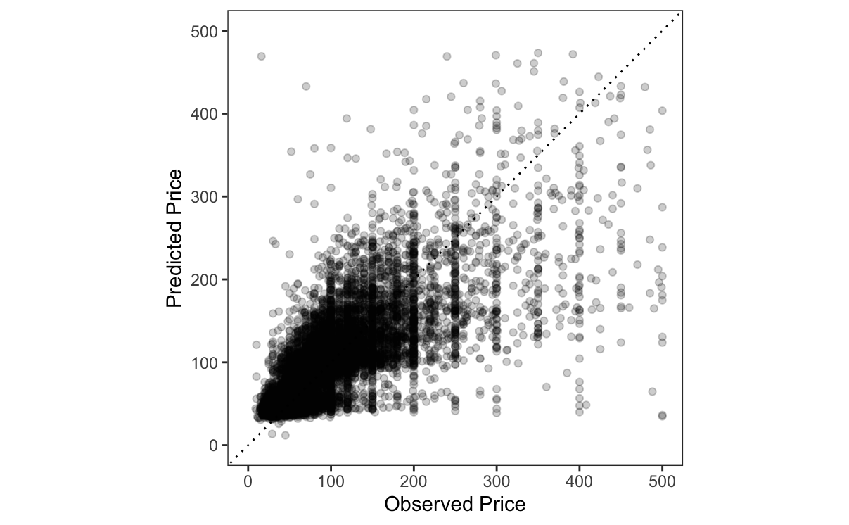
p=predictions(mod, newdata =test)ggplot(p, aes(x =price, y =estimate))+geom_point(alpha =.2)+geom_abline(linetype =3)+labs(x ="Observed Price", y ="Predicted Price")+xlim(0, 500)+ylim(0, 500)+coord_equal()
Figure 13.1: XGBoost predictions of rental prices against observed prices.
Every point in Figure 13.1 represents one rental unit in the test set. The x-axis shows the observed price for that unit, and the y-axis shows the predicted price. Points on the diagonal are correctly predicted. There is considerable spread around that diagonal, which means our algorithm makes substantial prediction errors.
Most of the standard functions and arguments in marginaleffects are available. For instance, to compute the average predicted price of private rooms and entire homes in the test set, we call avg_predictions() with the by argument.3
Unsurprisingly, our model expects that, on average, entire homes should be more expensive than private rooms.
13.2.1 Partial dependence plot
A Partial Dependence Plot (PDP) is a strategy to visualize how predictions change with certain predictors. It computes predictions over a range of values for a predictor, averaging over other variables, to show how outcomes vary with changes in a feature. This is useful for understanding complex models.
The plot_predictions() function in the marginaleffects package simplifies the creation of these plots. The command below computes average predicted outcomes for each combination of bedrooms and unit_type, and plots the results.
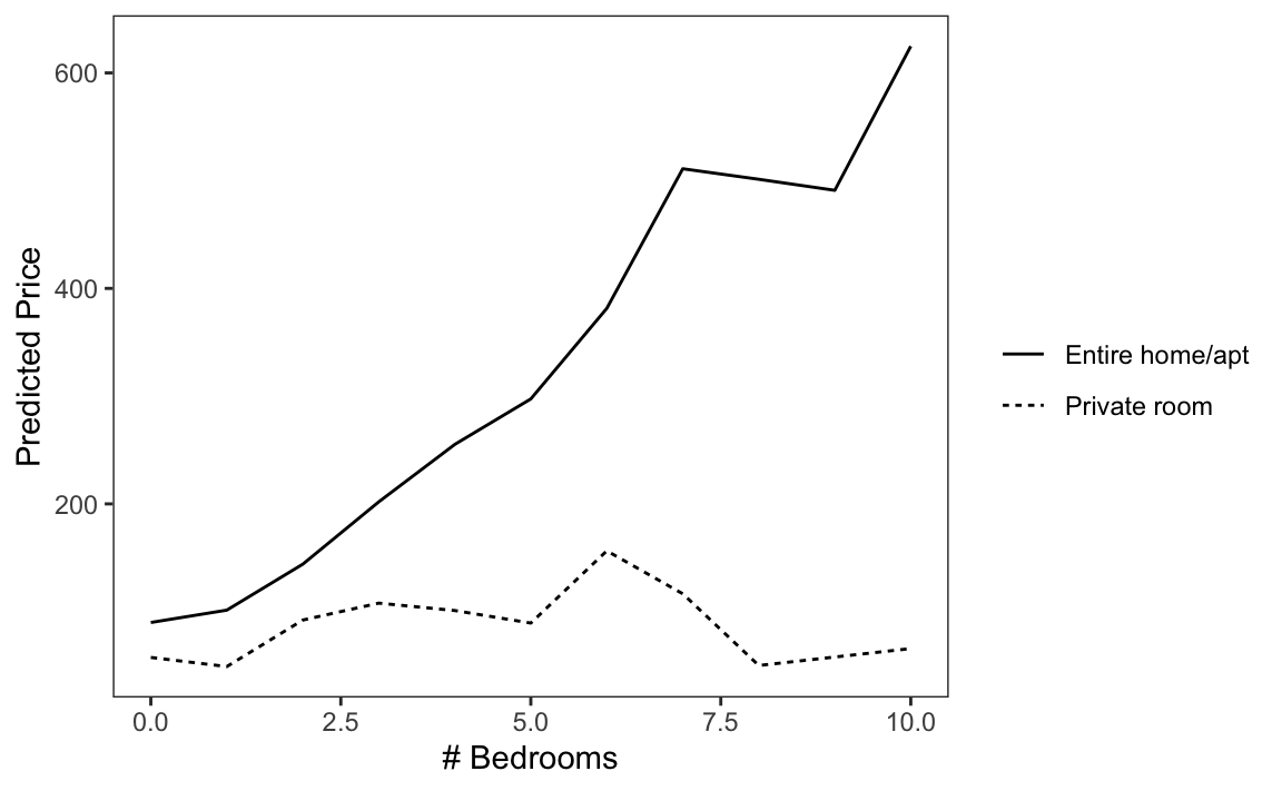
plot_predictions(mod, by =c("bedrooms", "unit_type"), newdata =airbnb)+labs(x ="# Bedrooms", y ="Predicted Price", linetype ="")
Figure 13.2: Relationship between predicted price, number of bedrooms, and type of rental unit in London.
The plot in Figure 13.2 makes sense substantively. On the one hand, the price of a single private room does not really change as we increase the total number of bedrooms in the unit. On the other, the price of renting an entire unit does increase with the number of bedrooms.
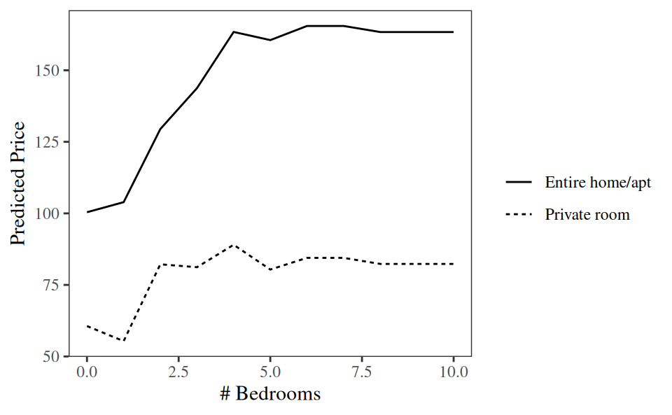
In some contexts, analysts prefer to draw partial dependence plots based on a counterfactual grid.4 The idea, here, is to duplicate the entire dataset once for every combination of values of the focal variables. Then, we make predictions on that counterfactual grid, and take an average of predictions. This counterfactual approach ensures that the distribution of marginalized covariates is identical for every combination of predictors. The resulting plots can be interpreted as illustrating “all else equal” predictions.
To draw this kind of partial dependence plot, we first build a counterfactual grid. If the data is very large, duplicating it several times to create counterfactual versions can require a lot of memory. To circumvent this problem, we build the grid based on random subset of 10,000 rows from the data set.
As in Chapter 6, we can use the avg_comparisons() function to answer counterfactual queries such as: On average, how does the predicted price change when we increase the number of bedrooms by 2, holding all other variables constant?
Our model predicts that the price of a unit with two extra bedrooms will be £27 higher. Furthermore, we may inquire about the combined effect of increasing the number of bedrooms by one, and of transitioning from an apartment without wireless internet access to one with such access. For this, we use the cross argument.
On average, adding one bedroom and wireless internet access to a rental unit increases the expected price by 15.
In conclusion, the integration of machine learning models with tools like marginaleffects allows for a deeper understanding and interpretation of complex models. By leveraging predictions, counterfactual comparisons, and partial dependence plots, analysts can gain insights into model behavior and ensure that predictions align with domain knowledge. This approach not only enhances model transparency but also aids in making informed decisions based on model outputs.
Békés, Gábor, and Gábor Kézdi. 2021. Data Analysis for Business, Economics, and Policy. Cambridge University Press. https://www.gabors-data-analysis.com.
Bischl, Bernd, Raphael Sonabend, Lars Kotthoff, and Michel Lang, eds. 2024. Applied Machine Learning Using Mlr3 in r. 1st ed. Chapman; Hall/CRC.
James, Gareth, Daniela Witten, Trevor Hastie, and Robert Tibshirani. 2023. An Introduction to Statistical Learning: With Applications in Python. 2023rd ed. Springer Nature.
Kuhn, Max, and Julia Silge. 2022. Tidy Modeling with r: A Framework for Modeling in the Tidyverse. 1st ed. O’Reilly Media.
Kuhn, Max, and Hadley Wickham. 2020. Tidymodels: A Collection of Packages for Modeling and Machine Learning Using Tidyverse Principles.https://www.tidymodels.org.
Lang, Michel, Martin Binder, Jakob Richter, et al. 2019. “mlr3: A Modern Object-Oriented Machine Learning Framework in R.”Journal of Open Source Software, ahead of print, December. https://doi.org/10.21105/joss.01903.
Pedregosa, F., G. Varoquaux, A. Gramfort, et al. 2011. “Scikit-Learn: Machine Learning in Python.”Journal of Machine Learning Research 12: 2825–30.
See Kuhn and Silge (2022), James et al. (2023), Bischl et al. (2024)↩︎
Note that when we apply a marginaleffects function to model fitted by tidymodels or mlr3, we do not obtain standard errors. This is because the parameters of machine learning estimates are not typically accompanied by a variance-covariance matrix, which implies that we cannot use the delta method. tidymodels has built-in support for some uncertainy quantification strategies like conformal prediction.↩︎