11  Mixed effects regression and post stratification

In this case study, we use mixed effects regression with post-stratification (MRP) to estimate the level of support, in each American State, for budget cuts to police forces.¹ This analysis, based on Ornstein (2023), has three main objectives.

First, this chapter shows how to use the marginaleffects package to interpret estimates obtained by fitting mixed effects regression models (aka, multilevel, hierarchical, or random effects models). Second, it demonstrates that a consistent post-estimation workflow can be applied to interpret the results of both frequentist and bayesian models. In the Bayesian case, marginaleffects is particularly useful, because it allows us to conduct prior and posterior predictive checks directly on the scale of the actual quantities of the interest. Finally, this case study illustrates how to implement post-stratification with marginaleffects, to account for unrepresentative sampling.

The data we consider was originally collected by the 2020 Cooperative Election Study (CES), and distributed by Ornstein (2023). The primary outcome, defund, is a binary variable which measures whether respondents support cuts to police budgets.² Predictors include individual-level covariates: gender, race, age, and education. The dataset also records if each survey respondent has been a member of the military, and which state they live in.

The survey data frame includes 3000 observations, randomly drawn from the full CES data.

survey <- readRDS("data/ces_survey.rds")
str(survey)

Classes 'data.table' and 'data.frame':  3000 obs. of  6 variables:
 $ state    : chr  "TX" "NJ" "CO" "PA" ...
 $ defund   : num  0 1 0 0 0 1 1 1 0 1 ...
 $ gender   : chr  "Woman" "Woman" "Woman" "Man" ...
 $ age      : Factor w/ 6 levels "18-29","30-39",..: 6 1 5 4 6 3 6 1 1 5 ...
 $ education: Factor w/ 6 levels "No HS","High school",..: 3 5 5 5 2 3 5 2 5 5 ...
 $ military : num  1 0 1 1 1 0 0 0 0 1 ...
 - attr(*, ".internal.selfref")=<externalptr> 

11.1 Mixed effects models

Mixed effects models are a popular strategy to study data that can be characterized as having a “hierarchical”, “nested”, or “multi-level” structure. Examples of nested data include survey respondents in different states; repeated measures made on the same subjects or on clustered observations; or students nested in classrooms, schools, districts, and states. A thorough introduction to mixed effects modeling lies outside the scope of this chapter, but interested readers can refer to many great texts on the subject (Gelman and Hill 2006; Finch, Bolin, and Kelley 2019; Bürkner 2024).

The parameters of a mixed effects model can be divided into two types: “fixed effects” and “random effects.” Fixed effects are parameters that are assumed to be constant across all groups in the population. Random effects, on the other hand, are parameters that are allowed to vary across groups. A major benefit of mixed effects models is thus that they allow variation in parameters between subsets of the data. For example, by specifying a “random intercept,” the analyst can let the baseline level of support for defund vary across US states. By including a “random slope” for the gender variable, they can allow the strength of association between gender and defund to vary from state to state.

Importantly, the random parameters of a mixed effects model are not completely free to vary from group to group. Instead, the model typically imposes constraints on the shape of the distribution of parameters. In effect, this “regularizes” the parameters, allowing estimates for groups with small sample sizes to be informed by estimates for groups with larger sample sizes. This can reduce the risk of overfitting and stabilize estimates for smaller groups.

11.2 Frequentist

Several software packages in R allow us to fit mixed effects models from a frequentist perspective, such as lme4 (Bates et al. 2015) and glmmTMB (Brooks et al. 2017). When using one of these packages, we define our models using the familiar formula syntax. The fixed components of our model are specified as we would any other predictor when fitting a linear or generalized linear model. Random effects components are specified using a special syntax with parentheses and a pipe | character.

y = x + (1 + z | group)

The formula above indicates that y is the outcome variable; the association between x and y is captured by a fixed effect parameter; 1 is a random intercept which allows the baseline level of y to vary across groups; z is a random slope, allowing the strength of association between z and y to vary across groups; and group is the grouping variable.

To model the probability of supporting cuts to police budgets, we use the glmmTMB package and fit a logistic regression model which includes a random intercept and random gender slope by state.

library(glmmTMB)
library(marginaleffects)

mod <- glmmTMB(
    defund ~ age + education + military + (1 + gender | state),
    family = binomial,
    data = survey)

summary(mod)

 Family: binomial  ( logit )
Formula:          defund ~ age + education + military + (1 + gender | state)
Data: survey

     AIC      BIC   logLik deviance df.resid 
  3824.7   3914.8  -1897.4   3794.7     2985 

Random effects:

Conditional model:
 Groups Name        Variance Std.Dev. Corr 
 state  (Intercept) 0.000757 0.02751       
        genderWoman 0.016493 0.12842  0.25 
Number of obs: 3000, groups:  state, 48

Conditional model:
                       Estimate Std. Error z value Pr(>|z|)    
(Intercept)           -0.149344   0.226237  -0.660  0.50918    
age30-39               0.010705   0.125542   0.085  0.93205    
age40-49              -0.788114   0.134194  -5.873 4.28e-09 ***
age50-59              -0.976043   0.127831  -7.635 2.25e-14 ***
age60-69              -1.184212   0.132270  -8.953  < 2e-16 ***
age70+                -1.387400   0.152823  -9.079  < 2e-16 ***
educationHigh school   0.090198   0.228857   0.394  0.69349    
educationSome college  0.408315   0.229887   1.776  0.07571 .  
education2 year        0.190178   0.247937   0.767  0.44306    
education4 year        0.603017   0.229599   2.626  0.00863 ** 
educationPost grad     0.958753   0.240669   3.984 6.78e-05 ***
military              -0.002505   0.082981  -0.030  0.97591    
---
Signif. codes:  0 '***' 0.001 '**' 0.01 '*' 0.05 '.' 0.1 ' ' 1

The signs of these estimated coefficients are interesting, but their magnitudes are somewhat difficult to interpret. As in previous chapters, we can use the marginaleffects package to make sense of those estimates.

To start, we use the predictions() function to compute the predicted probability of supporting cuts to police budgets for two hypothetical individuals: one from California, and one from Alabama.³

p <- predictions(mod, newdata = datagrid(
    state = c("CA", "AL"),
    gender = "Man",
    military = 0,
    education = "4 year",
    age = "50-59"
))
p

state	gender	military	education	age	Estimate	Std. Error	z	Pr(>|z|)	2.5 %	97.5 %
CA	Man	0	4 year	50-59	0.377	0.0295	12.8		0.319	0.435
AL	Man	0	4 year	50-59	0.372	0.0294	12.7		0.315	0.430

Our model predicts that a survey respondent with these demographic characteristics has a 37.7% chance of supporting funding cuts if they live in California, but a 37.2% chance if they live in Alabama.

To assess the strength of association between age and defund, we can use the avg_comparisons() function:

avg_comparisons(mod, variables = "age")

Contrast	Estimate	Std. Error	z	Pr(>|z|)	2.5 %	97.5 %
mean(30-39) - mean(18-29)	0.00257	0.0302	0.0853	0.932	-0.0566	0.0617
mean(40-49) - mean(18-29)	-0.18971	0.0313	-6.0529		-0.2511	-0.1283
mean(50-59) - mean(18-29)	-0.23178	0.0292	-7.9457		-0.2890	-0.1746
mean(60-69) - mean(18-29)	-0.27549	0.0290	-9.4953		-0.3324	-0.2186
mean(70+) - mean(18-29)	-0.31476	0.0313	-10.0531		-0.3761	-0.2534

The age of survey respondents is strongly related to their propensity to answer “yes” on the defund question. On average, our model predicts that moving from the younger age bracket (18-29) to the older one (70+) is associated with a reduction of 31 percentage points in the probability of supporting cuts to police staff.

This brief example shows that we can apply the same workflow described in earlier chapters to interpet the results of mixed effects models. In the next section, we analyze a similar model from a Bayesian perspective.

11.3 Bayesian

Bayesian regression analysis has a long history in statistics. Recent developments in computing, algorithm design, and software development have dramatically lowered the barriers to entry; they have made it much easier for analysts to estimate bayesian mixed effects models.⁴

A typical bayesian analysis involves several (often iterative) steps, including model formulation, prior specification, model refinement, estimation, and interpretation. Together, these steps form a “bayesian workflow” that allows analysts to go from data to insight (Gelman et al. 2020).

This section illustrates how to use the brms package for R to fit bayesian mixed effects models, and how the marginaleffects package facilitates two important steps of the bayesian workflow: prior predictive checks and posterior summaries.

The model that we consider here has the same basic structure as the frequentist model from the previous section. Expressed in terms of an R formula, it takes this form:

defund ~ age + education + military + (1 + gender | state),

The age, education, and military variables are associated to fixed effect parameters, while the gender and intercept parameters are allowed to vary from state to state.

11.3.1 Prior predictive checks

One important difference between bayesian and frequentist analysts, is that the former must explicitly specify priors over the parameters of their model. These priors can encode prior knowledge, beliefs, or information about the parameters in question. Some priors can have an important impact on the results of the analysis, so it is crucial to choose them carefully.

Using the priors function from the brms package for R, we can easily specify different priors. For example, if there is a lot of uncertainty about the value of the parameters in our model, we can set “vague” or “diffuse” priors, say from a normal distribution with a large variance:

library(brms)
library(ggdist)

priors_vague = c(
  prior(normal(0, 1e6), class = "b"),
  prior(normal(0, 1e6), class = "Intercept")
)

In contrast, if the analyst is confident that the parameters should be closer to zero, they can choose a more informative (narrow) prior:

priors_informative = c(
  prior(normal(0, 0.2), class = "b"),
  prior(normal(0, 0.2), class = "Intercept")
)

For many analysts, choosing priors is a difficult exercise. Part of this difficulty is linked to the fact that we are often required to specify priors for parameters that are expressed on an unintuitive scale (Chapter 4). What do the coefficients of a mixed-effect logit model mean, and does it make sense to think that they are distributed normally with a variance of 0.1?

To help answer this question, we can conduct prior predictive checks, that is, we can simulate quantities of interest from the pure model and priors, without considering any data at all. This allows us to check if different priors make sense, by looking at simulated quantities of interest that may have more intuitive interpretations than raw coefficients. On the basis of those results, we can refine the model purely based on our prior knowledge, before we let our views be influenced by the observed data.

To conduct a prior predictive check in R, we begin by using the brm() function and its formula syntax to specify the model structure, with fixed and random parameters. Then, we set family=bernoulli to estimate a logistic regression model. We use the prior argument to specify the priors we want to use. In this case study, we will consider “vague” and “informative” priors in turn. Finally, we set sample_prior="only" to tell brms to ignore the dataset altogether, and to draw simulations only from priors.

model_vague <- brm(
    defund ~ age + education + military + (1 + gender | state),
    family = bernoulli,
    prior = priors_vague,
    sample_prior = "only",
    data = survey)

model_informative <- brm(
    defund ~ age + education + military + (1 + gender | state),
    family = bernoulli,
    prior = priors_informative,
    sample_prior = "only",
    data = survey)

The sample_prior option is powerful. It allows to draw simulated coefficients from the model and priors, without looking at the data. But one problem remains: the results of this prior predictive check are still expressed on the same unintuitive scale as the model parameters:

fixef(model_vague)

                         Estimate Est.Error     Q2.5   Q97.5
Intercept               -64.52817 1277118.6 -2503669 2470353
age30M39              12224.98124  965172.9 -1905308 1903391
age40M49              -5000.48459  999100.8 -1976481 2006828
age50M59             -22431.75970  990874.1 -1922450 1840329
age60M69              -7307.01693 1002583.5 -1981705 1925807
age70P                 2783.08557 1024596.0 -2017230 2018742
educationHighschool   -7875.14159 1002754.8 -1978310 1919583
educationSomecollege    374.18454 1001792.5 -1957266 1904321
education2year        10045.30795  987896.1 -1929747 1966257
education4year        13818.10795 1004540.4 -1982538 1974888
educationPostgrad     -5467.56215  981028.2 -1962918 1943607
military              -3931.51836 1003751.9 -1902693 1939522

How can we know if these priors and the simulated results? One simple approach is to post-process prior-only brms model using marginaleffects. Using this strategy, we can compute any of the quantities of interest introduced earlier in this book, using only the information encoded by the model structure and prior distributions.

For example, when we adopt vague priors, the average predicted value of defund for each gender is:

avg_predictions(model_vague, by = "gender")

gender	Estimate	2.5 %	97.5 %
Man	0.501	0.0322	0.972
Woman	0.503	0.0342	0.971

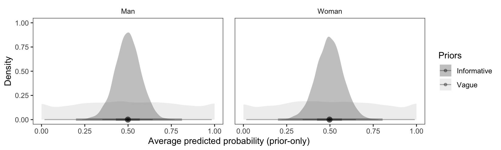
When using vague normal priors, the average predicted probability of supporting cuts to police budgets is centered at zero, with credible intervals that cover nearly the full \([0,1]\) interval. Unsurprisingly, the intervals are narrower when we use informative priors:

avg_predictions(model_informative, by = "gender")

gender	Estimate	2.5 %	97.5 %
Man	0.501	0.356	0.636
Woman	0.503	0.346	0.655

If the ultimate goal of our analysis is to compute an average treatment effect via G-Computation (Chapters 7 and ?sec-gcomputation), we can conduct a prior predictive check directly on that quantity. Once again, the intervals are much wider when using vague priors:

avg_comparisons(model_vague, variables = "military")

Estimate	2.5 %	97.5 %
0	-0.555	0.56

avg_comparisons(model_informative, variables = "military")

Estimate	2.5 %	97.5 %
-0.000416	-0.0594	0.0579

11.3.2 Posterior summaries

Instead of specifying our own priors, we now fit the model to data using the default priors set up by the brms package for this kind of model:

model <- brm(
    defund ~ age + education + military + (1 + gender | state),
    family = bernoulli,
    data = survey)

Using this model, we consider the average predicted probability of respondent defund=1 for respondents of either gender. By default, marginaleffects functions report the mean of posterior draws, along with compute the mean of the posterior distribution of draws, along with equal-tailed intervals:

p <- avg_predictions(model, by = "military")
p

military	Estimate	2.5 %	97.5 %
0	0.448	0.424	0.472
1	0.364	0.341	0.387

On average, people who are not part of the military have a 44.8% chance of supporting cuts to police budgets. In contrast, survey respondents with military backgrounds have, on average, an estimated probability of 36.4% chance.

As in Chapter 7, we can use the avg_comparisons() function to assess the strength of association between age and defund:

avg_comparisons(model, variables = list(age = c("18-29", "70+")))

On average, holding all other variables constant at their observed values, moving from the 18-29 to the 70+ age categories would be associated with a decrease of 31.4 percentage points in the probability of supporting funding cuts.

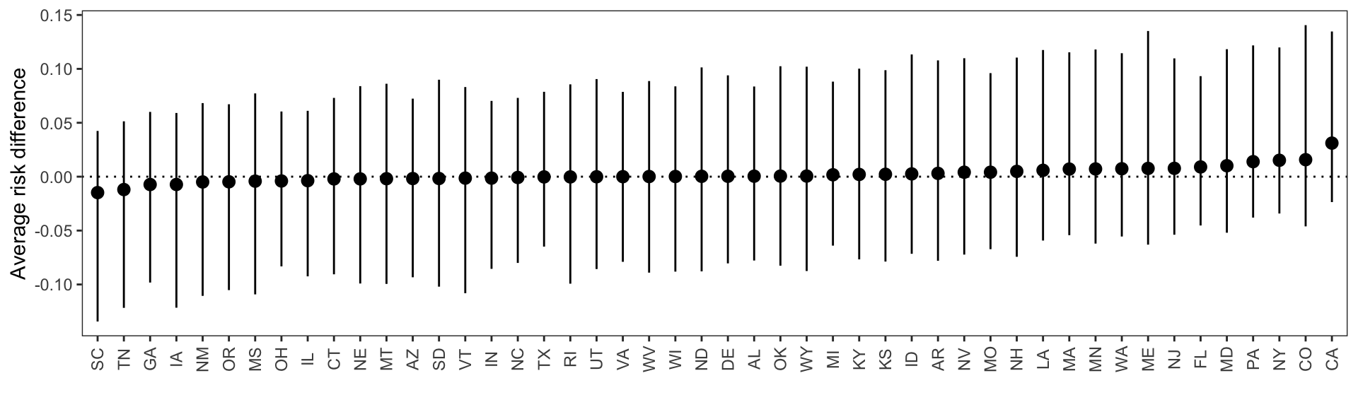
Recall that, in our model specification, we allowed the parameter associated to gender to vary from state to state. This means that our model could let the association between gender and defund to vary from state to state. Let’s see if this is the case.

First, we call the comparisons() function with the newdata argument to compute risk differences for one individual per state, whose characteristics are set to the average or mode of the predictors:

cmp <- comparisons(model,
    variables = "gender", 
    newdata = datagrid(state = unique))

Then, we sort the data, convert the state variable to a factor to preserve that order, and call ggplot to display the results:

cmp <- sort_by(cmp, ~estimate) |>
    transform(state = factor(state, levels = state))

ggplot(cmp, aes(y = estimate, ymin = conf.low, ymax = conf.high, x = state )) +
    geom_hline(yintercept = 0, linetype = 3) +
    geom_pointrange() + 
    labs(x = "", y = "Average risk difference") +
    theme(axis.text.x = element_text(angle = 90, vjust = .5))

Figure 11.1: Average risk difference for a hypothetical individual with typical characteristics living in different states.

The results in Figure 11.1 suggest that when we consider a hypothetical individual with mean or modal characteristics, risk difference in defund for different values of gender is very stable across states: it hovers around zero.

When post-processing bayesian results, it is often useful to directly manipulate draws from the posterior distribution. To extract these draws, we can use the posterior_draws() function. This function can return several different types of objects, including data frames in “wide” or “long” formats, matrices, or as a rvar distribution object compatible with the posterior package. For instance, we can print the first 5 draws from the posterior distribution of average predictions with:

draws <- avg_predictions(model) |> posterior_draws(shape = "long")
draws[1:5, 1:2]

  drawid      draw
1      1 0.4041124
2      2 0.4102879
3      3 0.4072840
4      4 0.4038716
5      5 0.4121313

This allows us to compute various posterior summaries using standard R functions. For example, we can see that about 71% of the posterior density of the average prediction lies above 0.4:

mean(draws$draw > .4)

[1] 0.706

11.4 Post-stratification

The sample that we used so far is relatively large: 3000 observations. But even if those observations were drawn randomly from the national population, they may still be insufficient to estimate state-level opinion. Indeed, some states are much more populous than others, and our dataset includes very few observations from certain areas of the country:

sort(tapply(survey$state, survey$state, length))

 ND  WY  SD  VT  MS  ID  MT  NE  NH  RI  DE  AR  KS  ME  WV  NM  OK  IA  NV  UT 
  4   5   8   9  12  14  14  15  15  15  19  21  21  21  21  22  23  32  32  33 
 KY  CT  LA  MN  OR  AL  MD  MA  WA  CO  SC  WI  TN  IN  MO  AZ  NJ  GA  VA  NC 
 40  42  44  44  46  47  49  53  57  59  60  67  70  76  76  81  88  90  90  91 
 MI  IL  OH  PA  NY  FL  TX  CA 
 94 107 136 144 180 224 224 265 

This kind of disparity occurs in many contexts, such as when one estimates quantities like:

• Presidential voting intentions in swing states, based on a national survey.
• Psychological well-being of a population, using a web-based survey that oversamples young and highly-educated people.
• Effect of a user interface change on website sales, based on an unbalanced sample of laptop or smartphone users.
• Vaccination rates using data from healthcare providers who are overrepresented in affluent neighborhoods.

To draw state-level inferences about defund, we will use the MRP approach, or mixed effects regression with poststratification. MRP is implemented in four steps:

1. Model Fitting: A model is developed to predict the outcome of interest (e.g., support for police reform) based on individual-level characteristics from the survey (e.g., gender, education, race, age). This model incorporates the hierarchical data structure, using techniques like mixed effects modeling to estimate varying intercepts for different states.
2. Constructing the Post-stratification Frame: A poststratification frame is created to represent the joint frequency distribution of predictor variables within each group of interest (e.g., proportions of men and women, age groups, education levels, and racial groups within each state). This information is typically sourced from the Census or other reliable data sets.
3. Predict and Poststratify: Using the fitted model, predicted probabilities for the outcome are generated for each cell in the poststratification frame (e.g., the predicted probability that a white, middle-aged woman in California supports police reform).
4. Weighted average: Compute a weighted average of these predicted probabilities is calculated using population weights from the poststratification frame to produce the final MRP estimates.

First, we estimate a mixed-effects model with random intercept by state. As Ornstein (2023) notes, the accuracy of MRP estimates depends on the predictive performance of this first-stage model, and may be affected by standard problems such as overfitting. Since we have already estimated such a model for previous examples, we simply use the same brms model object as before: model.

Second, we construct the post-stratification frame, that is, a dataset that contains information about the prevalence of each possible predictor profile. In our case, the demographics post-stratification frame records the prevalence of socio-demographic characteristics for each state:⁵

demographics <- readRDS("data/ces_demographics.rds")
head(demographics)

    state    age   education gender military   percent
   <char> <fctr>      <fctr> <char>    <num>     <num>
1:     AL  18-29       No HS    Man        0 0.3181336
2:     AL  18-29       No HS    Man        1 0.2120891
3:     AL  18-29       No HS  Woman        0 0.5302227
4:     AL  18-29       No HS  Woman        1 0.3181336
5:     AL  18-29 High school    Man        0 1.8027572
6:     AL  18-29 High school    Man        1 0.6362672

This table shows, for example, that about 0.318% of the Alabama population are women between the ages of 18 and 29, with no high school degree, and no military experience.

The third step in MRP is to make predictions for each row of the poststratification frame. In other words, we use the demographics data frame as a grid instead of the empirical grid:

p <- predictions(model, newdata = demographics)

Finally, we take a weighted average of these predictions by state, where weights are defined as the proportion of each demographic group in the state’s population. To do this with marginaleffects, we modify the call above, specifying weights with the wts argument, and the aggregation unit with the by argument:

p <- avg_predictions(model, 
  newdata = demographics,
  wts = "percent",
  by = "state")
head(p)

state	Estimate	2.5 %	97.5 %
AL	0.407	0.353	0.460
AR	0.397	0.344	0.463
AZ	0.379	0.332	0.427
CA	0.454	0.413	0.502
CO	0.437	0.396	0.507
CT	0.402	0.350	0.452

This command gives us one estimate per state. After adjusting for the demographic composition of the state of Alabama, our model estimates that the average probability of supporting cuts to police budgets is 40.7%, with a 95% credible interval of [35.3, 46.0].

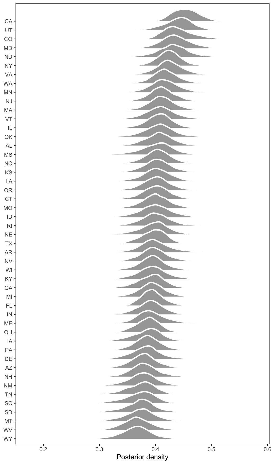
To visualize the results, we can extract draws from the posterior distribution using the posterior_draws() function, and use the ggdist package to plot densities. Figure 11.2 shows that the support for cuts to police budgets varies across states, with highest estimates in California and lowers in Wyoming.

library(ggdist)
library(ggplot2)

p <- p |>
  posterior_draws(shape = "rvar") |>
  sort_by(~ estimate) |>
  transform(state = factor(state, levels = state))

ggplot(p, aes(y = state, xdist = rvar)) + 
  stat_slab(height = 2, color = "white") +
  labs(x = "Posterior density", y = NULL)

Figure 11.2: Estimated average probability of supporting cuts to police budgets, for each US state. Estimates obtained via Bayesian multi-level regression and post-stratification.

Bates, Douglas, Martin Mächler, Ben Bolker, and Steve Walker. 2015. “Fitting Linear Mixed-Effects Models Using lme4.” Journal of Statistical Software 67 (1): 1–48. https://doi.org/10.18637/jss.v067.i01.

Brooks, Mollie E., Kasper Kristensen, Koen J. van Benthem, Arni Magnusson, Casper W. Berg, Anders Nielsen, Hans J. Skaug, Martin Maechler, and Benjamin M. Bolker. 2017. “glmmTMB Balances Speed and Flexibility Among Packages for Zero-Inflated Generalized Linear Mixed Modeling.” The R Journal 9 (2): 378–400. https://doi.org/10.32614/RJ-2017-066.

Bürkner, Paul C. 2024. The Brms Book: Applied Bayesian Regression Modelling Using r and Stan (Early Draft). https://paulbuerkner.com/software/brms-book.

Finch, W Holmes, Jocelyn E Bolin, and Ken Kelley. 2019. Multilevel Modeling Using r. Chapman; Hall/CRC.

Gelman, Andrew, John B. Carlin, Hal S. Stern, David B. Dunson, Aki Vehtari, and Donald B. Rubin. 2013. Bayesian Data Analysis. 3rd ed. New York: Chapman; Hall/CRC. https://doi.org/10.1201/b16018.

Gelman, Andrew, and Jennifer Hill. 2006. Data Analysis Using Regression and Multilevel/Hierarchical Models. 1st ed. Cambridge University Press. http://www.stat.columbia.edu/~gelman/arm/.

Gelman, Andrew, Aki Vehtari, Daniel Simpson, Charles C. Margossian, Bob Carpenter, Yuling Yao, Lauren Kennedy, Jonah Gabry, Paul-Christian Bürkner, and Martin Modrák. 2020. “Bayesian Workflow.” https://arxiv.org/abs/2011.01808.

McElreath, Richard. 2020. Statistical Rethinking: A Bayesian Course with Examples in r and STAN. 2nd ed. New York: Chapman; Hall/CRC. https://doi.org/10.1201/9780429029608.

Ornstein, Joseph T. 2023. “Getting the Most Out of Surveys: Multilevel Regression and Poststratification.” In Causality in Policy Studies: A Pluralist Toolbox, edited by Alessia Damonte and Fedra Negri, 99–122. Springer. https://doi.org/10.1007/978-3-031-12982-7_5.

---

1. This case study only includes code for R. The features illustrated here are on the roadmap for Python, but they are not supported yet.

2. The survey firm asked respondents if they supported or opposed this policy: “Decrease the number of police on the street by 10 percent, and increase funding for other public services.”

3. Note that the uncertainty estimates reported by marginaleffects for frequentist mixed effects models only take into account the variability in fixed effects parameters, and not in random effects parameters. As we will see below, bayesian modeling allows for more options in the quantification of uncertainy.

4. A comprehensive treatment of bayesian modeling would obviously require more space than this short chapter affords. Interested readers can refer to many recent texts, such as Gelman et al. (2013), McElreath (2020) or Bürkner (2024).

5. Ideally, the demographics data frame would be “complete”, in the sense that it would record the prevalence of every possible type of individual, in every state. Unfortunately, this is not always possible, when demographic information is not available for certain subsets of the population, for example in narrow groups, in less populous states.