7 Slopes
A slope measures how the predicted value of the outcome \(Y\) responds to changes in a focal predictor \(X\), when we hold other covariates at fixed values. It is often the main quantity of interest in an empirical analysis, when a researcher wants to estimate an effect or the strength of association between two variables. Slopes belong to the same toolbox as the counterfactual comparisons explored in Chapter 6. Both quantities help us answer a counterfactual query: What would happen to a predicted outcome if one of the predictors were slightly different?
One challenge in understanding slopes is that they are formally defined in the language of calculus. This chapter does not dive deep into theory. It focuses on intuition, eschews most technical details, and provides graphical examples to make abstract ideas more tangible. Nevertheless, readers who are not comfortable with the basics of multivariable calculus may want to jump ahead to the case studies in the next part of this book.
Beyond the technical barriers, another factor that hinders our understanding of slopes is that the terminology used talk about them is woefully inconsistent. In some fields, like economics or political science, slopes are called “marginal effects,” where the word “marginal” refers to the effect of an infinitesimal change in a focal predictor. In other disciplines, a slope may be called a “trend,” “velocity,” or “partial effect.” Some analysts even use the term “slope” when they write about the raw parameters of a regression model.
In this book, we use the expressions “slope” and “marginal effect” interchangeably to mean:
Partial derivative of the regression equation with respect to a predictor of interest.
Consider a simple linear model with outcome \(Y\) and predictor \(X\).
\[ Y = \beta_0 + \beta_1 X +\varepsilon \\ \tag{7.1}\]
To find the slope of \(Y\) with respect to \(X\), we take the partial derivative.
\[ \frac{\partial Y}{\partial X} = \beta_1 \tag{7.2}\]
The slope of Equation 7.1 with respect to \(X\) is thus equivalent to \(\beta_1\), the only coefficient in the equation. This identity explains why some analysts refer to regression coefficients as slopes. It also gives us a clue for interpretation.
In simple linear models, a one-unit increase in \(X\) is associated with a \(\beta_1\) change in \(Y\), holding other modelled covariates constant. Likewise, we will often be able to interpret the slope, \(\frac{\partial Y}{\partial X}\), as the effect of a one-unit change in \(X\) on the predicted value of \(Y\). This interpretation is useful as a first cut, but it comes with caveats.
First, given that slopes are defined as derivatives, that is, in terms of an infinitesimal change in \(X\), they can only be constructed for continuous numeric predictors. Analysts who are interested in the effect of a change in a categorical predictor should turn to counterfactual comparisons.1
Second, the partial derivative measures the slope of \(Y\)’s tangent at a specific point in the predictor space. Thus, the interpretation of a slope as the effect of a one-unit change in \(X\) must be understood as an approximation, valid in a small neighborhood of the predictors, for a small change in \(X\). This approximation may not be particularly good when the regression function is non-linear, or when the scale of \(X\) is small.
Finally, the foregoing discussion implies that slopes are conditional quantities, in the sense that they typically depend on the value of \(X\), but also on the values of all the other predictors in a model. Every row of a dataset or grid has its own slope. In that respect, slopes are like the predictions and counterfactual comparisons from chapters 5 and 6.
The rest of this chapter proceeds as before, by answering the five questions of our conceptual framework: (1) quantity, (2) predictors, (3) aggregation, (4) uncertainty, and (5) test.
7.1 Quantity
A slope characterizes the strength and the direction of association between a predictor and an outcome, holding other covariates constant. To get an intuitive feel for what this means in practice, it is useful to consider a few graphical examples. In this section, we will see that the slope of a curve tells us how it behaves as we move from left to right along the x-axis, that is, it tells us whether the curve is increasing, decreasing, or flat. This information is useful to understand the relationships between variables of interest in a regression model.
7.1.1 Slopes of simple functions
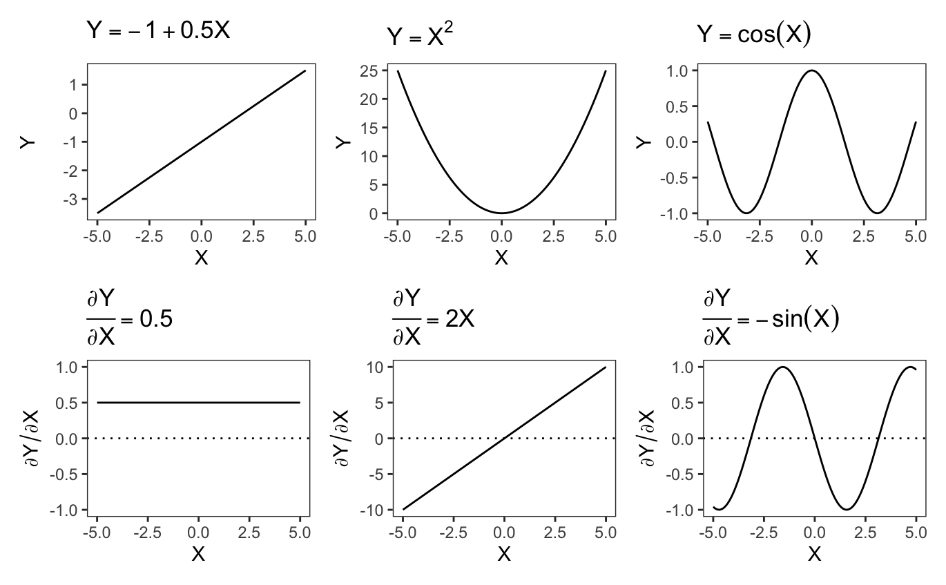
The top row of Figure 7.1 shows three functions of \(X\). The bottom row traces the derivatives of each of those functions. By examining the values of derivatives at any given point, we can determine precisely where the corresponding functions are rising, falling, or flat.
First, consider the top left panel of Figure 7.1, which displays the function \(Y=-1+0.5X\), a straight line with a positive slope. As we move from left to right, the line steadily rises. The effect of \(X\) is constant across the full range of \(X\) values. For every one-unit increase in \(X\), \(Y\) increases by 0.5 units. Since the slope does not change, the derivative of this function is constant (bottom left panel): \(\frac{\partial Y}{\partial X} = 0.5.\) This means that the association between \(X\) and \(Y\) is always positive, and that the strength of association between \(X\) and \(Y\) is of constant magnitude, regardless of the baseline value of \(X\).
Now, consider the top middle panel of Figure 7.1, which displays the function \(Y = X^2\), a symmetric parabola that opens upward. As we move from left to right, the function initially decreases, until it reaches its minimum at \(X=0\). In the left part of the plot, the relationship between \(X\) and \(Y\) is negative: an increase in \(X\) is associated to a decrease in \(Y\). When \(X\) reaches 0, the curve becomes flat: the slope of its tangent line is zero. This means that an infinitesimal change in \(X\) would have (essentially) no effect on \(Y\). As \(X\) continues to increase beyond zero, the function starts increasing, with a positive slope. The derivative of this function captures this behavior. When \(X<0\), the derivative is \(\frac{\partial Y}{\partial X}=2X<0\), which indicates that the relationship between \(X\) and \(Y\) is negative. When \(X=0\), the derivative is \(2X=0\), which means that the association between \(X\) and \(Y\) is null. When the \(X>0\), the derivative is positive, which implies that an increase in \(X\) is associated with an increase in \(Y\). In short, the sign and strength of the relationship between \(X\) and \(Y\) are heterogeneous; they depend on the baseline value of \(X\). This will be an important insight to keep in mind for the case study in Chapter 10, where we explore the use of interactions and polynomials to study heterogeneity and non-linearity.
The third function in Figure 7.1, \(Y = \cos(X)\), oscillates between positive and negative values, forming a wave-like curve. Focusing on the first section of this curve, we see that \(\cos(X)\) decreases as we move from left to right, reaches a minimum at \(-\pi\), and then increases until \(X=0\). The derivative plotted in the bottom right panel captures this trajectory well. Indeed, whenever \(-\sin(X)\) is negative, we see that \(\cos(X)\) points downward. When \(-\sin(X)=0\), the \(\cos(X)\) curve is flat and reaches a minimum or a maximum. When \(-\sin(X)>0\), the \(\cos(X)\) function points upward.
These three examples show that the derivative of a function precisely characterizes both the strength and the direction of association between a predictor and an outcome. It tells us, at any given point in the predictor space, if increasing \(X\) should result in a decrease or an increase in \(Y\).
7.1.2 Slope of a logistic function
Let us now consider a more realistic example, similar to the curves we are likely to fit in an applied regression context.
\[ Pr(Y=1) = g\left (\beta_1 + \beta_2 X \right), \tag{7.3}\]
where \(g\) is the logistic function, \(\beta_1\) is an intercept, \(\beta_2\) a regression coefficient, and \(X\) is a numeric predictor. Imagine that the true parameters are \(\beta_1=-1\) and \(\beta_2=0.5\). We can simulate a dataset with a million observations that follow this data generating process.
library(marginaleffects)
library(patchwork)
set.seed(48103)
N = 1e6
X = rnorm(N, sd = 2)
p = plogis(-1 + 0.5 * X)
Y = rbinom(N, 1, p)
dat = data.frame(Y, X)
Now, we fit a logistic regression model with the glm() function and print the coefficient estimates.
The estimated coefficients are very close to the true values we encoded in the data-generating process.
To visualize the outcome function and its derivative, we use the plot_predictions() and plot_slopes() functions. The latter is very similar to the plot_comparisons() function introduced in Section 6.6. The variables argument identifies the focal predictor with respect to which we are computing the slope, and the condition argument specifies which variable should be displayed on the x-axis. To display plots on top of one another, we use the / operator supplied by the patchwork package.
p_function = plot_predictions(mod, condition = "X")
p_derivative = plot_slopes(mod, variables = "X", condition = "X")
p_function / p_derivative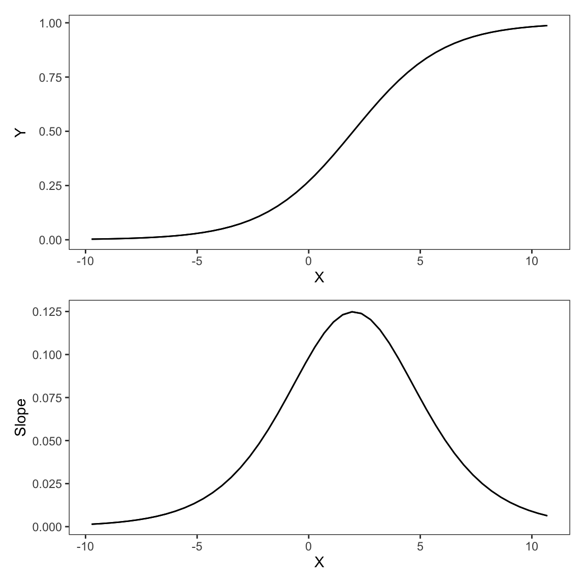
The key insight from Figure 7.2 is that the slope of the logistic function is far from constant. Increasing \(X\), moving from left to right on the graph, has a different effect on the estimated probability that \(Y=1\), depending on our position on the horizontal axis. When the initial value of \(X\) is small (left side of the figure), an increase in \(X\) results in a small change in \(Pr(Y=1)\): the prediction curve is relatively flat and the derivative is close to zero. At intermediate values of \(X\) (middle of the figure), a change in \(X\) results in a large increase in \(Pr(Y=1)\): the outcome prediction curve is steep, and its derivative is positive and large. When the initial value of \(X\) is large (right side of the figure), a change in \(X\) does not change \(Pr(Y=1)\) much: the outcome curve is flat and the derivative small again. In sum, the slope characterizes the strength of association between \(X\) and \(Y\) for different baseline values of the predictors.
To estimate the slope, we can proceed analytically, using the chain rule of differentiation. Taking the derivative of Equation 7.3 with respect to \(X\) gives us
\[ \frac{\partial Pr(Y=1)}{\partial X} = \beta_2 \cdot g'(\beta_1 + \beta_2 X), \tag{7.4}\]
where \(g'\) is the logistic density function, or the derivative of \(g\).2 To obtain an estimate of the slope, we simply plug-in our coefficient estimates into Equation 7.4. Importantly, whenever we evaluate a slope, we must explicitly state the baseline values of the predictors of interest. The slope of \(Y\) with respect to \(X\) will be different when \(X\) takes on different values. For example, the estimated \(\frac{\partial Pr(Y=1)}{\partial X}\) for \(X\in \{-5, 0, 10\}\) are
data.frame(
  "dY/dX|X=-5" = b[2] * dlogis(b[1] + b[2] * -5),
  "dY/dX|X=0" = b[2] * dlogis(b[1] + b[2] * 0),
  "dY/dX|X=10" = b[2] * dlogis(b[1] + b[2] * 10)
)
dY/dX|X=-5 dY/dX|X=0 dY/dX|X=10
0.0142749 0.09827211 0.008856198Alternatively, we could compute the same estimates with the slopes() function from marginaleffects. slopes() is very similar to the comparisons() function introduced in Chapter 6. The variables argument specifies the focal predictor, and newdata specifies the values of the other predictors at which we want to evaluate the slope.
| X | Estimate | Std. Error | z | Pr(>|z|) | 2.5 % | 97.5 % |
|---|---|---|---|---|---|---|
| -5 | 0.01427 | 7.24e-05 | 197.0 | <0.001 | 0.01413 | 0.01442 |
| 0 | 0.09827 | 2.61e-04 | 376.6 | <0.001 | 0.09776 | 0.09878 |
| 10 | 0.00886 | 8.98e-05 | 98.6 | <0.001 | 0.00868 | 0.00903 |
The numeric estimates obtained for this contrived example are extremely similar to those we computed analytically, which is expected. In the rest of this chapter, we will explore how to use slopes() and its siblings avg_slopes() and plot_slopes(), to estimate and visualize a variety of slope-related quantities of interest.
For illustration, we will look at a variation on a model considered in previous chapters, using data from Thornton (2008). As before, the dependent variable is a dummy variable called outcome, equal to 1 if a study participant sought to learn their HIV status at a test center, and 0 otherwise. Since we are studying partial derivatives, the focal predictor must be a continuous numeric variable. Here, we choose distance, a measure the distance between the participant’s residence and the test center. Our model also includes incentive, a binary variable which we treat as a control.
The model we specify includes multiplicative interactions between incentive, distance, and its square. These interactions give the model a bit more flexibility to detect non-linear patterns in the data, but their real purpose is pedagogical: they show that the post-estimation workflow introduced in previous chapters can be applied in straightforward fashion to more complex models. Once again, we will ignore individual parameter estimates, and focus on quantities of interest with more intuitive substantive meanings.
dat = get_dataset("thornton")
mod = glm(outcome ~ incentive * distance * I(distance^2),
  data = dat, family = binomial)
summary(mod)
Coefficients:
                                 Estimate Std. Error z value Pr(>|z|)
(Intercept)                       0.42793    0.38264   1.118   0.2634
incentive                         1.79455    0.47386   3.787   <0.001
distance                         -1.48974    0.63658  -2.340   0.0193
I(distance^2)                     0.56304    0.29767   1.891   0.0586
incentive:distance                0.49785    0.76074   0.654   0.5128
incentive:I(distance^2)          -0.25193    0.34657  -0.727   0.4673
distance:I(distance^2)           -0.06694    0.03981  -1.682   0.0926
incentive:distance:I(distance^2)  0.03426    0.04544   0.754   0.4509
7.2 Predictors
Slopes can help us answer questions such as:
How does the predicted outcome \(\hat{Y}\) change when the focal variable \(X\) increases by a small amount and the adjustment variables \(Z_1, Z_2, \ldots, Z_n\) are held at specific values?
Answering questions like this requires us to select both the focal variable and the values of the adjustment variables where we want to evaluate the slope.
7.2.1 Focal variable
The focal variable is the predictor of interest. It is the variable whose association with (or effect on) \(Y\) we wish to estimate. The focal variable is the predictor in the denominator of the partial derivative notation \(\frac{\partial Y}{\partial X}\).
The slopes() function accepts a variables argument, which serves to specify a focal predictor. For example, the following code estimates the partial derivative of the outcome equation encoded in the mod object, with respect to the distance focal predictor.
slopes(mod, variables = "distance")7.2.2 Adjustment variables
Slopes are conditional quantities, in the sense that they typically depend on the values of all the variables on the right-hand side of a regression equation. Thus, every predictor profile—or combination of predictor values—will be associated with its own slope. Every row in a grid will have its own slope. Section 3.2 described different grids of predictor values, that is, different combinations of unit characteristics that could be of interest.
One common type of grid is the “interesting” or “user-specified” grid, which collects combinations of predictor values that hold particular scientific or domain-specific interest. For example, imagine that we are specifically interested in measuring the association between distance and outcome for an individual who is part of the treatment group (incentive is 1) and who lives at a distance of 1 from the test center. We can use the datagrid() helper function to specify a grid of interesting predictor values, and then pass that grid to the newdata argument of the slopes() function. The function will then return a “slope at user-specified values” or “marginal effect at interesting values.”
library(marginaleffects)
slopes(mod,
  variables = "distance",
newdata = datagrid(incentive = 1, distance = 1))| incentive | distance | Estimate | Std. Error | z | Pr(>|z|) | 2.5 % | 97.5 % |
|---|---|---|---|---|---|---|---|
| 1 | 1 | -0.0694 | 0.021 | -3.3 | <0.001 | -0.111 | -0.0282 |
Our model suggests that for an individual with baseline characteristics incentive=1 and distance=1, a one-unit increase in distance is associated with a decrease of about 6.9 percentage points in the probability that a study participant will seek to learn their HIV status. This interpretation is authorized by the fact that the printed estimate corresponds to the slope of the tangent of the outcome curve at the specified point in the predictor space. But it is important to remember that this interpretation is a linear approximation, only valid for small changes in the focal predictor.
Instead of manually specifying the baseline values of all predictors, we can set newdata="mean" to compute a “marginal effect at the mean” or a “marginal effect at representative values.” This is the slope of the regression equation with respect to the focal predictor, for an individual whose characteristics are exactly average (or modal) on all predictors.
slopes(mod, variables = "distance", newdata = "mean")| Estimate | Std. Error | z | Pr(>|z|) | 2.5 % | 97.5 % |
|---|---|---|---|---|---|
| -0.024 | 0.0135 | -1.77 | 0.0763 | -0.0505 | 0.00254 |
As noted in previous chapters, computing estimates at the mean is computationally efficient, but it may not be particularly informative when the perfectly average individual is not realistic or substantively interesting. The choice of reporting a slope at the mean may seem innocuous, but it is not. In fact, our slope at the mean is quite different from the slope that we computed above for specified values of the covariates: -0.024 vs. -0.069, or about a third of the size. This emphasizes the crucial importance of grid definition.
Finally, instead of computing slopes for just a few profiles, we can get them for every observation in the original sample. These “unit-level marginal effects” or “partial effects” are the default output of the slopes() function.
slopes(mod, variables = "distance")| Estimate | Std. Error | z | Pr(>|z|) | 2.5 % | 97.5 % |
|---|---|---|---|---|---|
| -0.23004 | 0.0915 | -2.5137 | 0.01195 | -0.4094 | -0.0507 |
| -0.16236 | 0.0598 | -2.7141 | 0.00665 | -0.2796 | -0.0451 |
| 0.00663 | 0.0290 | 0.2281 | 0.81956 | -0.0503 | 0.0635 |
| 0.00895 | 0.0326 | 0.2743 | 0.78382 | -0.0550 | 0.0729 |
| -0.06896 | 0.0278 | -2.4823 | 0.01305 | -0.1234 | -0.0145 |
| 2815 rows omitted | 2815 rows omitted | 2815 rows omitted | 2815 rows omitted | 2815 rows omitted | 2815 rows omitted |
| -0.05763 | 0.0165 | -3.4844 | < 0.001 | -0.0900 | -0.0252 |
| -0.07078 | 0.0216 | -3.2796 | 0.00104 | -0.1131 | -0.0285 |
| -0.05771 | 0.0166 | -3.4854 | < 0.001 | -0.0902 | -0.0253 |
| -0.04587 | 0.0132 | -3.4651 | < 0.001 | -0.0718 | -0.0199 |
| -0.00147 | 0.0160 | -0.0922 | 0.92651 | -0.0328 | 0.0298 |
7.3 Aggregation
A dataset with one marginal effect estimate per unit of observation is a bit unwieldy and difficult to interpret. Instead of presenting a large set of estimates, many analysts prefer to report the “average marginal effect” (or “average slope”), that is, the average of all the unit-level estimates. The average slope can be obtained in two steps, by computing unit-level estimates and then their average. However, it is more convenient to call the avg_slopes() function.
avg_slopes(mod, variables = "distance")| Estimate | Std. Error | z | Pr(>|z|) | 2.5 % | 97.5 % |
|---|---|---|---|---|---|
| -0.0516 | 0.00919 | -5.61 | <0.001 | -0.0696 | -0.0335 |
Note that there is a nuanced distinction to be drawn between the “marginal effect at the mean” shown in the previous section, and the “average marginal effect” presented here. The former is calculated based on a single individual whose characteristics are exactly average or modal in every dimension. The latter is calculated by taking the average of slopes for all the observed data points in the dataset used to fit a model. These two options will not always be equivalent; they can yield numerically and substantively different results. In general, the marginal effect at the mean might be useful when there are computational constraints. The average marginal effect will be useful when the dataset adequately represents the distribution of predictors in the population, in which case marginalizing across the distribution can give us a good one-number summary.
Sometimes, the average slope ignores important patterns in the data. For instance, we can imagine that distance has a different effect on outcome for individuals who receive a monetary incentive and for those who do not. To explore this kind of heterogeneity in the association between independent and dependent variables, we can use the by argument. This will compute “conditional average marginal effects”, or average slopes by subgroup.
The following results, for instance, show the average slope (strength of association) between distance and the probability that a study participant will travel to the clinic to learn their test result.
avg_slopes(mod, variables = "distance", by = "incentive")| incentive | Estimate | Std. Error | z | Pr(>|z|) | 2.5 % | 97.5 % |
|---|---|---|---|---|---|---|
| 0 | -0.0818 | 0.02464 | -3.32 | <0.001 | -0.1301 | -0.0335 |
| 1 | -0.0430 | 0.00952 | -4.52 | <0.001 | -0.0617 | -0.0244 |
Indeed, it seems that distance discourages travel to the clinic for individuals in both groups, but that the strength of the negative association between distance and outcome is stronger when incentive=0. In Section 7.5, we will formally test if the difference between these estimates is statistically significant.
7.4 Uncertainty
As with all other quantities estimated thus far, we can compute estimates of uncertainty around slopes using various strategies: Classical or robust standard errors, bootstrapping, simulation-based inference, etc. To do this, we use the vcov and conf_level arguments, or the inferences() function. Here are two simple examples: the first command clusters standard errors by village, while the second applies a non-parametric bootstrap.
avg_slopes(mod, variables = "distance", vcov = ~village)| Estimate | Std. Error | z | Pr(>|z|) | 2.5 % | 97.5 % |
|---|---|---|---|---|---|
| -0.0516 | 0.0112 | -4.61 | <0.001 | -0.0734 | -0.0297 |
avg_slopes(mod, variables = "distance") |> inferences(method = "boot")| Estimate | 2.5 % | 97.5 % |
|---|---|---|
| -0.0516 | -0.0676 | -0.0339 |
The estimates are the same, but the confidence intervals differ, depending on the uncertainty quantification strategy.
7.5 Test
Chapter 4 explained how to conduct complex null hypothesis tests on any quantity estimated by the marginaleffects package. The approach introduced in that chapter is applicable to slopes, as it was to model coefficients, predictions, and counterfactual comparisons.
Recall the example from Section 7.3, where we computed the average slopes of outcome with respect to distance, for each incentive subgroup.
avg_slopes(mod,
variables = "distance",
by = "incentive")| incentive | Estimate | Std. Error | z | Pr(>|z|) | 2.5 % | 97.5 % |
|---|---|---|---|---|---|---|
| 0 | -0.0818 | 0.02464 | -3.32 | <0.001 | -0.1301 | -0.0335 |
| 1 | -0.0430 | 0.00952 | -4.52 | <0.001 | -0.0617 | -0.0244 |
At first glance, these two estimates appear different. It seems that distance is more discouraging to people who do not receive an incentive. One might thus infer that money can mitigate the barrier posed by distance.
To ensure that this observation is not simply the product of sampling variation, we must formally check if the two estimates in the table are statistically distinguishable. To do this, we execute the same command as before, but add a hypothesis argument with an equation-like string. That equation specifies our null hypothesis: there is no difference between the first estimate (b1) and the second (b2).
avg_slopes(mod,
  variables = "distance",
  by = "incentive",
hypothesis = "b1 - b2 = 0")| Hypothesis | Estimate | Std. Error | z | Pr(>|z|) | 2.5 % | 97.5 % |
|---|---|---|---|---|---|---|
| b1-b2=0 | -0.0388 | 0.0264 | -1.47 | 0.142 | -0.0905 | 0.013 |
The difference between our two estimates is about -0.039, which suggests that the slope is flatter in the group with incentive. In other words, the association between distance and outcome is weaker when incentive=1 than when incentive=0. However, this difference is not statistically significant (\(p\)=0.142). Therefore, we cannot reject the null hypothesis of homogeneity in the effect of distance on the predicted probability that participants will seek their test results.
7.6 Visualization
When interpreting the results obtained by fitting a model, it is important to keep in mind the distinction between predictions and slopes. Predictions give us the level of an expected outcome, for given values of the predictors. Slopes capture how the expected outcome changes in response to a change in a focal variable, while holding adjustment variables constant. Figure 7.3 illustrates these concepts in two panels.
The top panel shows model-based predictions for the outcome variable at different values of distance, while holding other predictors at their mean or mode. As we move from left to right along the x-axis, as distance from the test center increases, the predicted probability of outcome=1 declines, flattens, and then declines again.
This pattern is mirrored in the bottom panel of Figure 7.3, which shows the slope of predicted outcome with respect to distance, holding adjustment variables at their mean or mode. For most values of distance, the slope is negative, which means that distance has a negative effect on the predicted probability that outcome equals 1. When distance is around 3 or 4, the association between distance and outcome is flat or null. At that point, small increases in distance no longer have much of an effect on predicted outcome. When the slope is below zero (dotted line), the prediction curve in the top panel goes down. When the slope is at zero, the prediction curve is flat.
To draw the two plots in Figure 7.3, we call the plot_predictions() and plot_slopes() functions, and combine the outputs in a single figure using the / operator from the patchwork package.
library(ggplot2)
library(patchwork)

p1 = plot_predictions(mod, condition = "distance") +
    labs(y = "Predicted Pr(Outcome=1)")

p2 = plot_slopes(mod, variables = "distance", condition = "distance") +
    geom_hline(yintercept = 0, linetype = "dotted") +
    labs(y = "dY/dX")

p1 / p2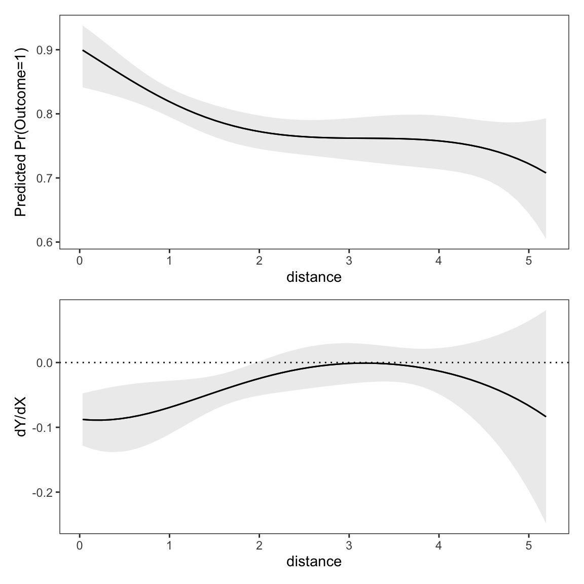
plot_slopes() can display several slopes based on multiple conditions. For example, we can show how the association between distance and outcome varies based on incentive and distance.
plot_slopes(mod,
  variables = "distance",
  condition = c("distance", "incentive"))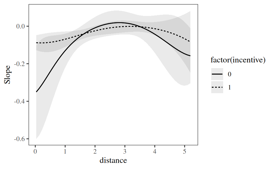
We can also compute marginal slopes, that is, the average of individual-level slopes by subgroup. To do this, we use the by argument. The next plot shows the same results we explored in Section 7.5. The negative association between distance and outcome seems weaker when incentive=1 than when incentive=0, but the confidence intervals are wide, so we cannot reject the null hypothesis that the two average slopes are equal.
plot_slopes(mod,
  variables = "distance",
  by = "incentive")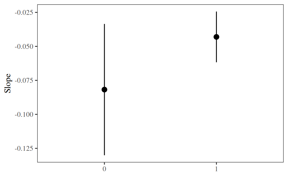
7.7 Summary
This chapter defined a “slope” as the partial derivative of the regression equation with respect to a predictor of interest. It is a measure of association between two variables, or of the effect of one variable on another, holding other predictors constant.
The slopes() function from the marginaleffects package computes slopes for a wide range of models. avg_slopes() aggregates slopes across units or groups. plot_slopes() displays slopes visually.
slopes(), avg_slopes(), and plot_slopes() functions.
| Argument | |
|---|---|
model |
Fitted model used to make counterfactual slopes. |
variables |
Focal predictor whose association with or effect on the outcome we are interested in. |
newdata |
Grid of predictor values. |
slope |
Choice between derivative or (semi-)elasticity. |
vcov |
Standard errors: Classical, robust, clustered, etc. |
conf_level |
Size of the confidence intervals. |
type |
Type of predictions to compare: response, link, etc. |
by |
Grouping variable for average predictions. |
wts |
Weights used to compute average slopes. |
hypothesis |
Compare different slopes to one another, conduct linear or non-linear hypothesis tests, or specify null hypotheses. |
equivalence |
Equivalence tests |
df |
Degrees of freedom for hypothesis tests. |
numderiv |
Algorithm used to compute numerical derivatives. |
... |
Additional arguments are passed to the predict() method supplied by the modeling package. |
To clearly define slopes and attendant tests, analysts must make five decisions.
First, the Quantity.
- A slope is always computed with respect to a focal predictor, whose effect on (or association with) the outcome we wish to estimate. In
marginaleffectsfunctions, the focal variable is specified using thevariablesargument. - A slope can roughly be interpreted as the effect of a one-unit change in the focal predictor on the predicted outcome. However, this interpretation is a linear approximation, valid only in a small neighborhood of the predictors.
Second, the Predictors.
- Slopes are conditional quantities, meaning that they will typically vary based on the values of all predictors in a model. Every row of a dataset has its own slope.
- Analysts can compute slopes for different combinations of predictor values—or grids: empirical, interesting, representative, balanced, or counterfactual.
- The predictor grid is defined by the
newdataargument and thedatagrid()function.
Third, the Aggregation.
- To simplify the presentation of results, analysts can report average slopes. Different aggregation schemes are available:
- Unit-level slopes (no aggregation)
- Average slopes
- Average slopes by subgroup
- Weighted average of slopes
- Slopes can be aggregated using the
avg_slopes()function and thebyargument.
Fourth, the Uncertainty.
- In
marginaleffects, thevcovargument allows analysts to report classical, robust, or clustered standard errors for slopes. - The
inferences()function can compute uncertainty intervals via bootstrapping or simulation-based inference.
Fifth, the Test.
- A null hypothesis test evaluates whether a slope (or a function of slopes) is significantly different from a null value. For example, we may use a null hypothesis test to check if treatment effects are equal in subgroups of the sample. Null hypothesis tests are conducted using the
hypothesisargument. - An equivalence test evaluates whether a slope (or a function of slopes) is similar to a reference value. Equivalence tests are conducted using the
equivalenceargument.