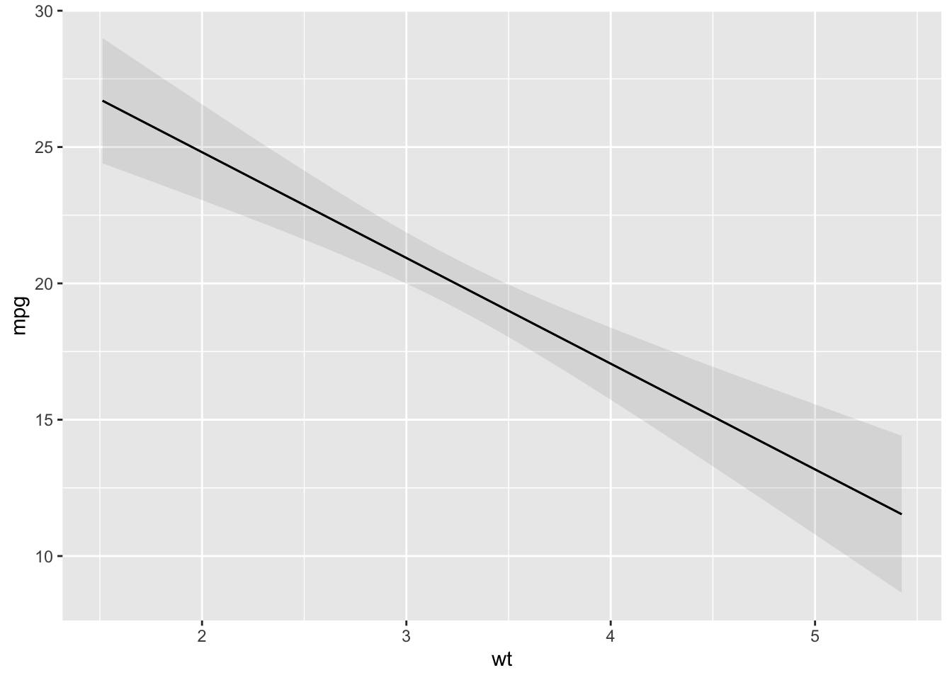
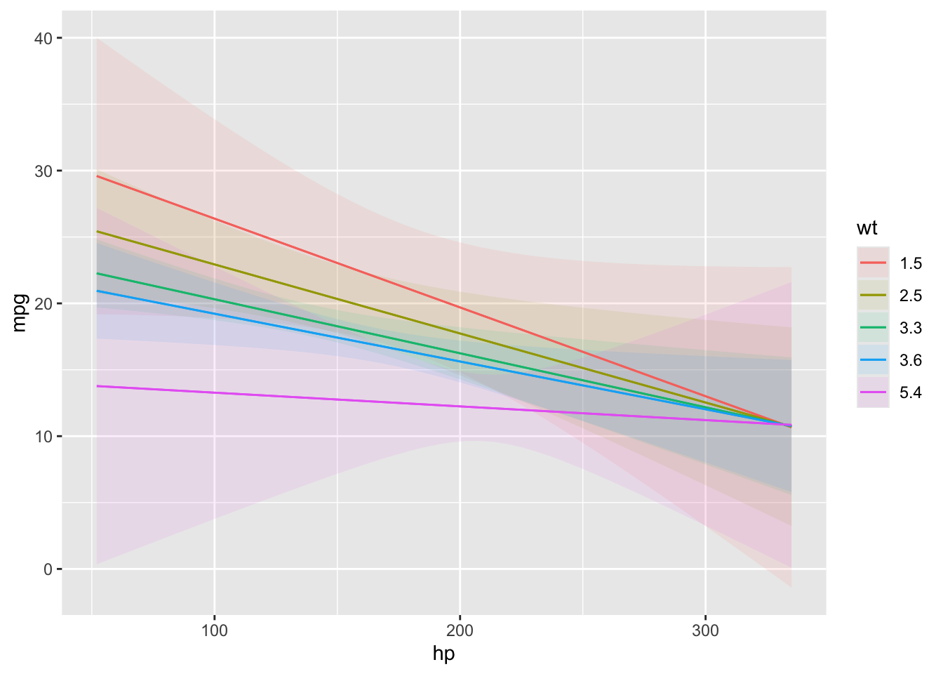
Plot Conditional or Marginal Predictions

Description

Plot predictions on the y-axis against values of one or more predictors (x-axis, colors/shapes, and facets).

The by argument is used to plot marginal predictions, that is, predictions made on the original data, but averaged by subgroups. This is analogous to using the by argument in the predictions() function.

The condition argument is used to plot conditional predictions, that is, predictions made on a user-specified grid. This is analogous to using the newdata argument and datagrid() function in a predictions() call. All variables whose values are not specified explicitly are treated as usual by datagrid(), that is, they are held at their mean or mode (or rounded mean for integers). This includes grouping variables in mixed-effects models, so analysts who fit such models may want to specify the groups of interest using the condition argument, or supply model-specific arguments to compute population-level estimates. See details below.

See the "Plots" vignette and website for tutorials and information on how to customize plots:

https://marginaleffects.com/bonus/plot.html
https://marginaleffects.com

Usage

plot_predictions(
  model,
  condition = NULL,
  by = NULL,
  newdata = NULL,
  type = NULL,
  vcov = NULL,
  conf_level = 0.95,
  wts = FALSE,
  transform = NULL,
  points = 0,
  rug = FALSE,
  gray = getOption("marginaleffects_plot_gray", default = FALSE),
  draw = TRUE,
  ...
)

Arguments

`model`	Model object
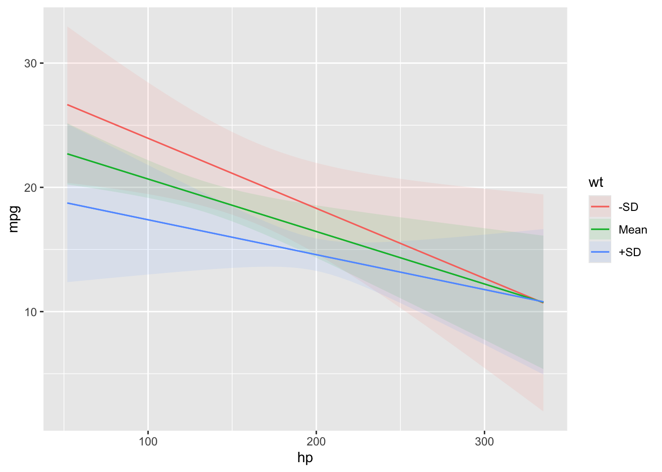
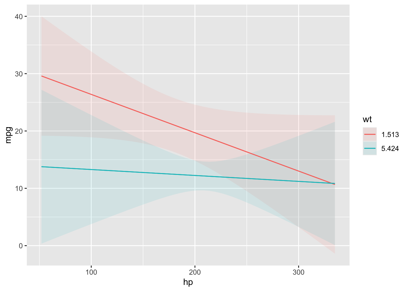
`condition`	Conditional predictions Character vector (max length 4): Names of the predictors to display. Named list (max length 4): List names correspond to predictors. List elements can be: Numeric vector Function which returns a numeric vector or a set of unique categorical values Shortcut strings for common reference values: "minmax", "quartile", "threenum" 1: x-axis. 2: color/shape. 3: facet (wrap if no fourth variable, otherwise cols of grid). 4: facet (rows of grid). Numeric variables in positions 2 and 3 are summarized by Tukey’s five numbers `?stats::fivenum`
`by`	Marginal predictions Character vector (max length 3): Names of the categorical predictors to marginalize across. 1: x-axis. 2: color. 3: facets.
`newdata`	When `newdata` is `NULL`, the grid is determined by the `condition` argument. When `newdata` is not `NULL`, the argument behaves in the same way as in the `predictions()` function.
`type`	string indicates the type (scale) of the predictions used to compute contrasts or slopes. This can differ based on the model type, but will typically be a string such as: "response", "link", "probs", or "zero". When an unsupported string is entered, the model-specific list of acceptable values is returned in an error message. When `type` is `NULL`, the first entry in the error message is used by default.
`vcov`	Type of uncertainty estimates to report (e.g., for robust standard errors). Acceptable values: FALSE: Do not compute standard errors. This can speed up computation considerably. TRUE: Unit-level standard errors using the default `vcov(model)` variance-covariance matrix. String which indicates the kind of uncertainty estimates to return. Heteroskedasticity-consistent: `“HC”`, `“HC0”`, `“HC1”`, `“HC2”`, `“HC3”`, `“HC4”`, `“HC4m”`, `“HC5”`. See `?sandwich::vcovHC` Heteroskedasticity and autocorrelation consistent: `“HAC”` Mixed-Models degrees of freedom: "satterthwaite", "kenward-roger" Other: `“NeweyWest”`, `“KernHAC”`, `“OPG”`. See the `sandwich` package documentation. One-sided formula which indicates the name of cluster variables (e.g., `~unit_id`). This formula is passed to the `cluster` argument of the `sandwich::vcovCL` function. Square covariance matrix Function which returns a covariance matrix (e.g., `stats::vcov(model)`)
`conf_level`	numeric value between 0 and 1. Confidence level to use to build a confidence interval.
`wts`	logical, string or numeric: weights to use when computing average predictions, contrasts or slopes. These weights only affect the averaging in `avg_*()` or with the `by` argument, and not unit-level estimates. See `?weighted.mean` string: column name of the weights variable in `newdata`. When supplying a column name to `wts`, it is recommended to supply the original data (including the weights variable) explicitly to `newdata`. numeric: vector of length equal to the number of rows in the original data or in `newdata` (if supplied). FALSE: Equal weights. TRUE: Extract weights from the fitted object with `insight::find_weights()` and use them when taking weighted averages of estimates. Warning: `newdata=datagrid()` returns a single average weight, which is equivalent to using `wts=FALSE`
`transform`	A function applied to unit-level adjusted predictions and confidence intervals just before the function returns results. For bayesian models, this function is applied to individual draws from the posterior distribution, before computing summaries.
`points`	Number between 0 and 1 which controls the transparency of raw data points. 0 (default) does not display any points. Warning: The points displayed are raw data, so the resulting plot is not a "partial residual plot."
`rug`	TRUE displays tick marks on the axes to mark the distribution of raw data.
`gray`	FALSE grayscale or color plot
`draw`	`TRUE` returns a `ggplot2` plot. `FALSE` returns a `data.frame` of the underlying data.
`…`	Additional arguments are passed to the `predict()` method supplied by the modeling package.These arguments are particularly useful for mixed-effects or bayesian models (see the online vignettes on the `marginaleffects` website). Available arguments can vary from model to model, depending on the range of supported arguments by each modeling package. See the "Model-Specific Arguments" section of the `?slopes` documentation for a non-exhaustive list of available arguments.

Value

A ggplot2 object or data frame (if draw=FALSE)

Model-Specific Arguments

Some model types allow model-specific arguments to modify the nature of marginal effects, predictions, marginal means, and contrasts. Please report other package-specific predict() arguments on Github so we can add them to the table below.

https://github.com/vincentarelbundock/marginaleffects/issues

Package	Class	Argument	Documentation
`brms`	`brmsfit`	`ndraws`	brms::posterior_predict
		`re_formula`	brms::posterior_predict
`lme4`	`merMod`	`re.form`	lme4::predict.merMod
		`allow.new.levels`	lme4::predict.merMod
`glmmTMB`	`glmmTMB`	`re.form`	glmmTMB::predict.glmmTMB
		`allow.new.levels`	glmmTMB::predict.glmmTMB
		`zitype`	glmmTMB::predict.glmmTMB
`mgcv`	`bam`	`exclude`	mgcv::predict.bam
	`gam`	`exclude`	mgcv::predict.gam
`robustlmm`	`rlmerMod`	`re.form`	robustlmm::predict.rlmerMod
		`allow.new.levels`	robustlmm::predict.rlmerMod
`MCMCglmm`	`MCMCglmm`	`ndraws`
`sampleSelection`	`selection`	`part`	sampleSelection::predict.selection

Prediction types

The type argument determines the scale of the predictions used to compute quantities of interest with functions from the marginaleffects package. Admissible values for type depend on the model object. When users specify an incorrect value for type, marginaleffects will raise an informative error with a list of valid type values for the specific model object. The first entry in the list in that error message is the default type.

The invlink(link) is a special type defined by marginaleffects. It is available for some (but not all) models, and only for the predictions() function. With this link type, we first compute predictions on the link scale, then we use the inverse link function to backtransform the predictions to the response scale. This is useful for models with non-linear link functions as it can ensure that confidence intervals stay within desirable bounds, ex: 0 to 1 for a logit model. Note that an average of estimates with type=“invlink(link)” will not always be equivalent to the average of estimates with type=“response”. This type is default when calling predictions(). It is available—but not default—when calling avg_predictions() or predictions() with the by argument.

Some of the most common type values are:

response, link, E, Ep, average, class, conditional, count, cum.prob, cumhaz, cumprob, density, detection, disp, ev, expected, expvalue, fitted, hazard, invlink(link), latent, latent_N, linear, linear.predictor, linpred, location, lp, mean, numeric, p, ppd, pr, precision, prediction, prob, probability, probs, quantile, risk, rmst, scale, survival, unconditional, utility, variance, xb, zero, zlink, zprob

Examples

library("marginaleffects")


mod <- lm(mpg ~ hp + wt, data = mtcars)
plot_predictions(mod, condition = "wt")

mod <- lm(mpg ~ hp * wt * am, data = mtcars)
plot_predictions(mod, condition = c("hp", "wt"))

plot_predictions(mod, condition = list("hp", wt = "threenum"))

plot_predictions(mod, condition = list("hp", wt = range))

# marginal predictions
mod <- lm(mpg ~ hp * am, data = mtcars)
plot_predictions(mod, by = "am")

# marginal predictions on a counterfactual grid
plot_predictions(mod,
  by = "am",
  newdata = datagrid(am = 0:1, grid_type = "counterfactual")
)