The main claim of this book is that the parameters of a statistical model are complex quantities that do not always have a straightforward meaning. Instead of trying to interpret them directly, we should treat parameters as a “resting stone on the way to prediction.”
In this chapter, we go further and show that predictions can themselves act as a springboard for further analysis. We will see how to combine predictions into counterfactual comparisons that quantify the strength of association between two variables, or the effect of a cause.
Counterfactual thinking is fundamental to scientific inquiry and data analysis. Indeed, many of our most important research questions can be expressed as comparisons between hypothetical worlds.
Would survival be more likely if patients received a new medication rather than a placebo?
Would standardized test scores be higher if class sizes were smaller?
Does participating in a micro-finance program increase household income?
Do conservation policies improve forest coverage?
To answer questions like these, researchers must conduct thought experiments. They must make counterfactual predictions, and then compare those predictions.
Say we want to estimate the effect of conservation policies on forest coverage. To start, we ask: what is the forest coverage in a region without conservation policies? Then, we ask: what would be the forest coverage in the same region, if conservation policies were implemented? Finally, we compare the two quantities: what is the difference between the expected forest coverage in counterfactual worlds with and without conservation policies?
In that spirit, we can define a broad class of quantities of interest:
A counterfactual comparison is a function of two or more model-based predictions, made with different predictor values.
This definition is intimately linked to the theories of causal inference surveyed in Section 2.1.3. As we will see, a natural way to estimate the effect of an intervention is to use a statistical model to make predictions in two counterfactual worlds and to compare those predictions. When the conditions for causal identification are satisfied, this counterfactual comparison can be interpreted as a measure of the effect of \(X\) on \(Y\).
But even where the conditions for causal identification are not satisfied, counterfactual comparisons remain very interesting statistical quantities. In that case, they can be treated as descriptive measures of the strength of association between two variables, holding other variables constant.
Sections 6.1 and 6.2 show that a vast array of estimands can be expressed as functions of two (or more) predictions: contrasts, risk differences, ratios, odds, lift, etc. Section 6.3 explains that we can aggregate counterfactual comparisons across different grids to compute quantities of interest like the average treatment effect (ATE) or the conditional average treatment effect (CATE). Section 6.4 discusses standard errors and confidence intervals, and Section 6.5 shows how we can contrast comparisons to one another, in view of exploring treatment effect heterogeneity. Section 6.6 concludes with some tips on data visualization.
6.1 Quantity
A counterfactual comparison is a function of two or more model-based predictions, made with different predictor values. To operationalize this quantity, we must make three decisions. First, what is the focal predictor whose effect on (or association with) the outcome we wish to estimate? Second, how does the focal predictor differ between counterfactual worlds? Third, what function do we use to compare predicted outcomes obtained for different values of the focal predictor?
To fix notation, consider a simple case where we fit a statistical model with outcome \(Y\) and focal predictor \(X\), and use the parameter estimates to compute predictions. When the variable \(X\) is set to a specific value \(x\), the model-based prediction is written \(\hat{Y}_{X=x}\).
An analyst who is interested in model description, data description, or causal inference may want to estimate how the predicted outcome \(\hat{Y}_{X}\) changes when we manipulate the predictor \(X\). For example, how does the predicted outcome change when \(X\) increases by 1 unit, by one standard deviation, or when \(X\) changes from one specific value to another?
\[\begin{align*}
\hat{Y}_{X=x+1} - \hat{Y}_{X=x} && \text{Increase of one unit}\\
\hat{Y}_{X=x+\sigma_X} - \hat{Y}_{X=x} && \text{Increase of one standard deviation}\\
\hat{Y}_{X=max(X)} - \hat{Y}_{X=min(X)} && \text{Increase from minimum to maximum}\\
\hat{Y}_{X=b} - \hat{Y}_{X=a} && \text{Change between specific values $a$ and $b$}
\end{align*}\]
In each of the examples above, we calculated the difference between two predicted outcomes, evaluated for different values of the focal predictor \(X\). A simple difference is often the best starting point for interpretation, because it is simple and easy to grasp intuitively. But we are not restricted to this function.
In the special case where the predicted outcome \(\hat{Y}_X\) is a probability, \(\hat{Y}_{X=b}-\hat{Y}_{X=a}\) is called a risk difference, \(\hat{Y}_{X=b}/\hat{Y}_{X=a}\) a risk ratio, and \(\frac{\hat{Y}_{X=b}}{1 - \hat{Y}_{X=b}} \bigg/ \frac{\hat{Y}_{X=a}}{1 - \hat{Y}_{X=a}}\) an odds ratio.
The rest of this chapter shows how to compute and interpret all of these quantities using the marginaleffects package.
For illustration, we fit a logistic regression model to data from Thornton (2008). The outcome is a binary variable which indicates if a study participant sought to learn their HIV status. The randomized treatment is a binary variable indicating whether the participant received a monetary incentive. To make the specification more flexible and improve precision, we interact the incentive indicator with two other predictors: a participant’s age category and their distance from the test center.
Optimization terminated successfully.
         Current function value: 0.535929
         Iterations 5
mod.summary()
Logit Regression Results
Dep. Variable:
outcome
No. Observations:
2825
Model:
Logit
Df Residuals:
2817
Method:
MLE
Df Model:
7
Date:
Mon, 13 Jul 2026
Pseudo R-squ.:
0.1324
Time:
11:25:57
Log-Likelihood:
-1514.0
converged:
True
LL-Null:
-1745.1
Covariance Type:
nonrobust
LLR p-value:
1.023e-95
coef
std err
z
P>|z|
[0.025
0.975]
Intercept
-0.4862
0.296
-1.641
0.101
-1.067
0.094
agecat[T.18 to 35]
0.0794
0.289
0.275
0.783
-0.487
0.645
agecat[T.>35]
0.3452
0.295
1.172
0.241
-0.232
0.923
incentive
2.0576
0.344
5.978
0.000
1.383
2.732
incentive:agecat[T.18 to 35]
-0.0585
0.335
-0.175
0.861
-0.715
0.598
incentive:agecat[T.>35]
-0.1247
0.342
-0.364
0.716
-0.796
0.546
distance
-0.1844
0.072
-2.548
0.011
-0.326
-0.043
incentive:distance
0.0230
0.083
0.279
0.780
-0.139
0.185
This is a simple logistic regression model. Yet, because the model includes interactions and a non-linear link function, interpreting raw model coefficients is difficult for most analysts, and essentially impossible for lay people.
Counterfactual comparisons are a compelling alternative to coefficient estimates, with many advantages for interpretation. First, counterfactual comparisons can be expressed directly on the scale of the outcome variable, rather than as complex functions like log-odds ratios. Second, counterfactual comparisons map directly onto what many people have in mind when they think of the effect of a treatment: what change can we expect in the outcome when a predictor changes? Finally, as the next sections show, the marginaleffects package makes it trivial to compute counterfactual comparisons. Data analysts can embrace the same workflow in model-agnostic fashion, applying similar post-estimation steps regardless of the kind of model they chose to estimate.
6.1.1 First steps: risk difference with a binary treatment
To begin, let us consider a simple estimand: the risk difference associated with a change in binary treatment. Specifically, we will estimate the expected change in outcome when the incentive variable is manipulated to equal 1 instead of 0.
An important factor to consider, when estimating such a quantity, is that counterfactual comparisons are conditional quantities. Except in the simplest cases, comparisons will depend on the values of all the predictors in a model. Each individual in a dataset may be associated with a different counterfactual comparison. Therefore, whenever the analyst computes a counterfactual comparison, they must explicitly define the values of the focal predictor, but also the values of all other covariates in the model.
Section 6.2 explores different ways to define a grid of predictor profiles. For now, we shall focus on a single individual with arbitrary characteristics.
Our goal is to estimate the risk difference for someone between the ages of 18 to 35, who lives a distance of 2 from the test center.
\[\hat{Y}_{i=1,d=2,a=\text{18 to 35}} - \hat{Y}_{i=0,d=2,a=\text{18 to 35}}\]
To compute this quantity, we must compare model-based predictions with and without the incentive, holding all other unit characteristics constant. Using simple base R commands, we manipulate the grid, make predictions, and compare those predictions.
The same estimate can be obtained more easily, along with standard errors and test statistics, using the comparisons() function from the marginaleffects package.
Our model suggests that, for a participant who is between 18 and 35 years old and lives a distance of 2 from the test center, moving from the control group to the treatment group increases the predicted probability that outcome equals one by \(0.465\times 100=46.5\) percentage points.
This result is interesting, but a note of caution is warranted. In this chapter, we will interpret the counterfactual comparison as a measure of the effect of a change in a focal predictor on the outcome predicted by a model. This is both a claim about the fitted model’s behavior,1 and a descriptive claim about the estimated association between a focal predictor and the outcome.2 To go further and give counterfactual comparisons a causal interpretation would require us to make strong assumptions. Chapter 8 discusses these assumptions in some detail.
6.1.2 Comparison functions
So far, we have measured the effect of a change in predictor solely by looking at differences in predicted outcomes. Differences are typically the best starting point for interpretation, because they are simple and easy to grasp intuitively. Nevertheless, in some contexts it can make sense to use different functions to compare counterfactual predictions, such as ratios, lift, or odds ratios.
To compute the ratio of predicted outcomes associated to a change in incentive, we use the comparison="ratio" argument.
The predicted outcome is nearly 2.5 times as large for a participant in the treatment group, who is between 18 and 35 years old and lives at a distance of 2 from the test center, than for a participant in the control group with the same socio-demographic characteristics. Note that, in the code above, we set hypothesis=1 to test against the null hypothesis that these two predicted probabilities are identical (ratio of 1). The standard error is small and the \(z\) statistic large.
Therefore, we can reject the null hypothesis that the predicted outcomes are the same in the treatment and control arms of this trial. We can reject the hypothesis that the ratio between the predicted probabilities that someone in the treatment group (incentive=1) and someone in the control group (incentive=0) will get their test results is 1.
To compute the lift, we would proceed in the same way, by setting comparison="lift".
Finally, it is useful to note that the comparison argument accepts arbitrary functions. This is an extremely powerful feature, as it allows analysts to specify fully customized comparisons between a hi prediction (e.g., treatment) and a lo prediction (e.g., control). To illustrate, we compute a log odds ratio based on average predictions.3
The predictors in a model can be divided in two categories: focal and adjustment variables. Focal variables are the key predictors in a counterfactual analysis. They are the variables whose effect on (or association with) the outcome we wish to quantify. In contrast, adjustment (or control) variables are incidental to the principal analysis. They can be included in a model to increase its flexibility, improve fit, control for confounders, or to check if treatment effects vary across subgroups of the population. However, the effect of an adjustment variable is not of inherent interest in a counterfactual analysis.4
As noted above, counterfactual comparisons are conditional quantities, which means that they typically depend on the values of all the predictors in a model. Therefore, when computing a comparison, we must decide where to evaluate it in the predictor space. We must decide what values to assign to both the focal and adjustment variables.
6.2.1 Focal variables
When estimating counterfactual comparisons, our goal is to determine what happens to the predicted outcome when one or more focal predictors change. Obviously, the kind of change we are interested in depends on the nature of the focal predictors. Let us consider four common cases: binary, categorical, numeric, and cross-comparisons.
For pedagogical purposes, we will treat each of the predictors in our model as a focal variable in turn: incentive, agecat, and distance. Note, however, that only the incentive variable was randomized in the Thornton (2008) study. In most real-world applications, there will only be one or two focal predictors per statistical model.5
6.2.1.1 Change in binary predictors
By default, when the focal predictor is binary, marginaleffects returns the value of the difference in predicted outcome associated to a change from the control (0) to the treatment (1) group.
Moving from the treatment to the control group on the incentive variable is a associated with a change of -47 percentage points in the predicted probability that outcome equals 1.
6.2.1.2 Change in categorical predictors
The same approach can be used when we are interested in changes in a categorical variable with multiple levels. For example, if we want to know how changes in the agecat variable affect the predicted probability that outcome equals 1, we use the variables argument.
Moving from the <18 category to the 18 to 35 category increases the predicted probability that outcome equals 1 by 0.4 percentage points. Moving from the <18 to the >35 age bracket increases the predicted probability by 3.6 percentage points.
By default, the comparisons() function returns comparisons between every level of the categorical predictor and its reference level, or first category. We can modify the variables argument to compare specific categories, or to compare all categories to its preceding level, sequentially: <18 to 18 to 35, and 18 to 35 to >35.
This table shows the effect of increasing distance by 1 unit on the predicted value of outcome. Importantly, this corresponds to an increase of 1 unit from the value of distance encoded in the predictor grid.
For a person between the ages of 18 and 35, in the treatment group, moving from 2 to 3 units on the distance variable is associated with a change of -2.9 percentage points on the predicted probability of the outcome.
One may be interested in different magnitudes of change in the focal predictor distance. For example, the effect of a 5 unit (or 1 standard deviation) increase in distance on the predicted value of the outcome. Alternatively, the analyst may want to assess the effect of a change between two specific values of distance, or across the interquartile (or full) range of the data. All of these options are easy to implement using the variables argument.
# Increase of 5 unitscomparisons(mod, variables =list("distance"=5), newdata =grid)# Increase of 1 standard deviationcomparisons(mod, variables =list("distance"="sd"), newdata =grid)# Change between specific valuescomparisons(mod, variables =list("distance"=c(0, 3)), newdata =grid)# Change across the interquartile rangecomparisons(mod, variables =list("distance"="iqr"), newdata =grid)# Change across the full rangecomparisons(mod, variables =list("distance"="minmax"), newdata =grid)
# Increase of 5 unitscomparisons(mod, variables={"distance": 5}, newdata=grid)# Increase of 1 standard deviationcomparisons(mod, variables={"distance": "sd"}, newdata=grid)# Change between specific valuescomparisons(mod, variables={"distance" : [0, 3]}, newdata=grid)# Change across the interquartile rangecomparisons(mod, variables={"distance" : "iqr"}, newdata=grid)# Change across the full rangecomparisons(mod, variables={"distance": "minmax"}, newdata=grid)
6.2.1.4 Cross-comparisons
Sometimes, an analyst wants to assess the joint or combined effect of manipulating two predictors. In a medical study, for example, we may be interested in the change in survival rates for people who both receive a new treatment and make a dietary change. In our running example, it may be interesting to know how much the predicted probability of outcome would change if we modified both the distance and incentive variables simultaneously. To check this, we use the cross argument.
These results show that a simultaneous increase of 1 unit in the distance variable and between 0 and 1 on the incentive variable is associated with a change of 0.437 in the predicted outcome.
6.2.2 Adjustment variables
In a typical counterfactual analysis, the researcher is not interested in a change in the adjustment variables themselves. Nevertheless, since the value of a counterfactual comparison depends on where it is evaluated in the predictor space, we must imperatively define the full grid of focal and adjustment variables.
Much like in Chapter 5, where we computed predictions for different profiles, we now estimate counterfactual comparisons on empirical, interesting, representative, and balanced grids.
6.2.2.1 Empirical distribution
By default, the comparisons() function returns estimates for every row of the original data frame that was used to fit the model. The Thornton (2008) dataset includes 2825 complete observations (after dropping missing data), so the next command will yield 2825 estimates.
If we do not specify the variables argument, comparisons() computes distinct differences for all the variables. Here, there are 4 possible differences, so we get \(4 \times 2825=11300\) rows.
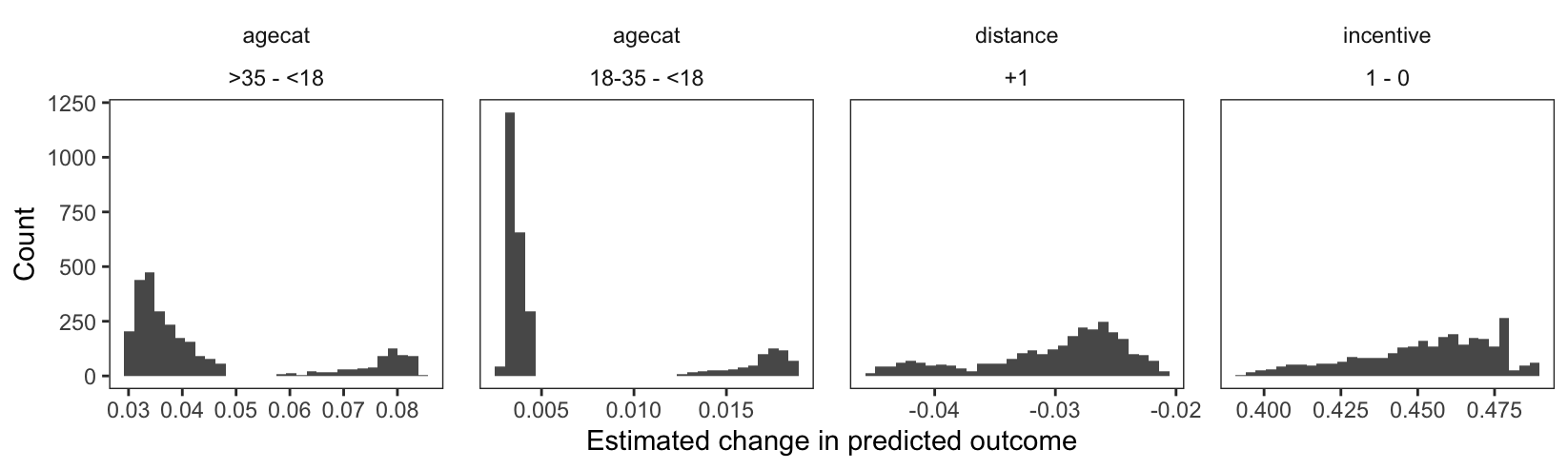
Figure 6.1: Distribution of unit-level risk differences associated with changes in each of the predictors.
The x-axes in Figure 6.1 show the estimated effects of changes in the predictors on the predicted value of the outcome. The y-axes show the prevalence of each estimate across the full sample.
There appears to be considerable heterogeneity. For example, consider the right-most panel, which plots the distribution of unit-level contrasts for the incentive variable. This panel shows that for some participants, the model predicts that moving from the control to the treatment condition would increase the predicted probability that outcome equals one by about 0.5 points. For others, the estimated effect of this change can be as low as 0.4.
6.2.2.2 Interesting grid
In some contexts, we want to estimate a contrast for a specific individual with characteristics of interest. To achieve this, we can supply a data frame to the newdata argument.
The code below shows the expected change in the predicted probability of the outcome associated with a change in incentive, for a few individuals with interesting characteristics. As in Chapter 5, we use the datagrid() function as a convenient mechanism to create a grid of profiles of interest.
Notice that the estimated effects of incentive on the predicted probability that outcome=1 differ depending on participants’ age. Indeed, our model estimates that the difference between treatment and control would be 46.6 percentage points in the central age category, but 43.8 percentage point in the older age category.
6.2.2.3 Representative grids
A common alternative is to compute a comparison or risk difference “at the mean.” The idea is to create a “representative” or “synthetic” profile for an individual whose characteristics are completely average or modal. Then, we report the comparison for this specific hypothetical individual. To do this, we use the “mean” shortcut in the newdata argument.
The main advantage of this approach is that it is fast and cheap from a computational standpoint. The disadvantage is that the interpretation is somewhat ambiguous. Often, the population includes no individual at all who is perfectly average across all dimensions and it is not always clear why we should be interested in such an individual. This matters because, in some cases, a “comparison at the mean” can differ significantly from an “average comparison.”6
6.2.2.4 Balanced grids
Balanced grids, introduced in Section 3.2, include all unique combinations of categorical variables, while holding numeric variables at their means. This is particularly useful in experimental contexts, where the sample is not representative of the target population, and where we want to treat each combination of treatment conditions similarly.
The code above converted the results to a data.frame. This is because marginaleffects automatically hides some columns when printing output. Calling as.data.frame() ensures that all columns are printed, which makes it easier to see the structure of the balanced grid.
6.3 Aggregation
As discussed above, the default behavior of comparisons() is to estimate quantities of interest for all the actually observed units in our dataset, or for each row of the dataset supplied to the newdata argument. Sometimes, it is convenient to marginalize those conditional estimates to obtain an average (or marginal) estimates.
Several key quantities of interest can be expressed as average counterfactual comparisons. For example, when certain assumptions are satisfied, the average treatment effect (ATE) of \(X\) on \(Y\) can be defined as the expected difference between outcomes under treatment or control:
\[
E[Y_{X=1} - Y_{X=0}],
\]
where the expectation is taken over the distribution of adjustment variables. In Chapter 8, we will see that estimands like the Average Treatment Effect on the Treated (ATT) or Average Treatment Effect on the Untreated (ATU) can be defined analogously.
To compute an average counterfactual comparison, we proceed in four steps:
Compute predictions for every row of the dataset in the counterfactual world where all observations belong to the treatment condition.
Compute predictions for every row of the dataset in the counterfactual world where all observations belong to the control condition.
Take the differences between the two vectors of predictions.
Average the unit-level estimates across the whole dataset, or within subgroups.
Previously, we called the comparisons() function to compute unit-level counterfactual comparisons. To return average estimates, we call the same function, with the same arguments, but add the avg_ prefix.
On average, across all participants in the study, moving from the control to the treatment group is associated with a change of 45.2 percentage points in the predicted probability that outcome equals one. This result is equivalent to computing unit-level estimates and taking their mean.
On average, for participants in the <18 age bracket, moving from the control to the treatment group is associated with a change of 47.5 percentage points in the predicted probability that outcome equals one. This average risk difference is estimated at 43.5 percentage points for participants above 35 years old.
We can also compute an average risk difference for individuals with specific profiles, by specifying the grid of predictors using the newdata argument. For example, if we are interested in an average treatment effect that only applies to study participants who actually belonged to the treatment group, we can call:7
Before moving on, it is useful to take a slight detour to highlight the relationships between three of the most important quantities of interest we have considered so far: average predictions, average counterfactual predictions, and average counterfactual comparisons.
To illustrate these concepts, we momentarily shift our focus to the Palmer Penguins dataset (Horst et al. 2020), which contains measurements of body mass and flipper lengths for three species of penguins: Adelie, Chinstrap, and Gentoo. On average, the dataset shows that Gentoo penguins are heaviest and have the longest flippers.
We fit a linear regression model to predict flipper length based on body mass and species. Average predictions are calculated over the observed distribution of covariates within each subset of interest. If Gentoo penguins are heavier than Adelie, that difference in predictors will be reflected in the average predictions.
Now, consider what happens when we compute average counterfactual predictions instead. As explained in Section 5.2.5, this involves duplicating the entire dataset three times—once for each penguin species—and fixing the focal variable to be constant in the three dataset. Then, we call the predict() and mean() functions from base R, in order to return the average expected flipper length.
Instead of this manual calculation, we can compute the average counterfactual predictions with the avg_predictions() function and its variables and by arguments.
Note that since we have replicated the full datasets, the distribution of body mass is now identical in all three datasets. By construction, the average counterfactual predictions are ceteris paribus quantities, that allow us to compare species while holding covariates constant. As a result of “ignoring” body mass, the gaps between average counterfactual predictions are smaller than the gaps between average predictions.
Finally, average counterfactual comparisons measure the differences between these counterfactual predictions, giving us the estimated effect of species on flipper length, while controlling for body mass. Average counterfactual comparisons can be computed directly by taking the difference between average counterfactual predictions, or by calling avg_comparisons().
This example illustrates how counterfactual predictions and comparisons allow us to conduct “all else equal” analyses—examining the relationship between variables while holding other factors constant. The differences between species are smaller in the counterfactual analysis than in the raw data because we have “controlled for” the fact that some species tend to be heavier than others.
In the next section, we go back to our running example.
6.4 Uncertainty
By default, the standard errors around contrasts are estimated using the delta method and the classical variance-covariance matrix supplied by the modeling software.8 For many of the more common statistical models, we can rely on the sandwich or clubSandwich packages to report “robust” standard errors, confidence intervals, and \(p\) values (Zeileis et al. 2020; Pustejovsky 2023). We can also use the inferences() function to compute bootstrap or simulation-based estimates of uncertainty.
Using the modelsummary package, we can report estimates with different uncertainty estimates in a single table, with models displayed side-by-side (Table 6.1).9
Table 6.1: Alternative ways to compute uncertainty about counterfactual comparisons.
Heteroskedasticity
Clustered
Bootstrap
agecat
18 to 35 - <18
0.0065
0.0065
0.0065
[-0.0457, 0.0587]
[-0.0468, 0.0599]
[-0.0475, 0.0562]
>35 - <18
0.0449
0.0449
0.0449
[-0.0079, 0.0977]
[-0.0033, 0.0931]
[-0.0065, 0.0932]
distance
+1
-0.0303
-0.0303
-0.0303
[-0.0427, -0.0179]
[-0.0449, -0.0157]
[-0.0422, -0.0186]
incentive
1 - 0
0.4519
0.4519
0.4519
[0.4110, 0.4928]
[0.4094, 0.4945]
[0.4116, 0.4933]
Num.Obs.
2825
2825
2825
6.5 Test
Earlier in this chapter, we estimated average counterfactual comparisons for different age subgroups. Now, we will see how to conduct hypothesis tests on these quantities, in order to compare them to one another.
Imagine one is interested in the following question:
Does moving from incentive=0 to incentive=1 have a bigger effect on the predicted probability that outcome=1 for older or younger participants?
To answer this, we can start by using the avg_comparisons() and its by argument to estimate sub-group specific average risk differences.
At first glance, it looks like the average counterfactual comparison is larger in the first age bin than in the last (0.475 vs. 0.435). It looks like the effect of incentive on the probability of seeking to learn one’s HIV status is stronger for younger participants than for older ones.
The difference between estimated treatment effects in those two groups is
\[
0.475 - 0.435 = 0.04,
\]
but is this difference statistically significant? Does our data allow us to conclude that incentive has different effects in age subgroups?
To answer this question, we follow the process laid out in Chapter 4, and express our test as a string formula, where b1 identifies the estimate in the first row and b3 in the third row.
There is a numerical difference between the two estimates, but the \(p\) value is large. This means that we cannot reject the null hypothesis that the effect of incentive on predicted outcome is the same for participants in the two age brackets. The two estimated risk differences are not statistically distinguishable from one another.
6.6 Visualization
In many cases, data analysts will want to visualize counterfactual comparisons rather than solely report numerical summaries. Figure 6.1 already showed how one could visualize unit-level comparisons. In this section, we will see how the plot_comparisons() can be used to visualize marginal and conditional comparisons.
6.6.1 Marginal comparisons
We already know that the avg_comparisons() function can be used to compute average counterfactual comparisons, or conditional average treatment effects by subgroups of the data. For example, it allows us to calculate the average change in predicted outcome associated with a change in incentive, for different age subgroups.
Instead of displaying these results in a table, we can call the plot_comparisons() function to compute the same estimates, and present them graphically. The syntax is nearly identical.
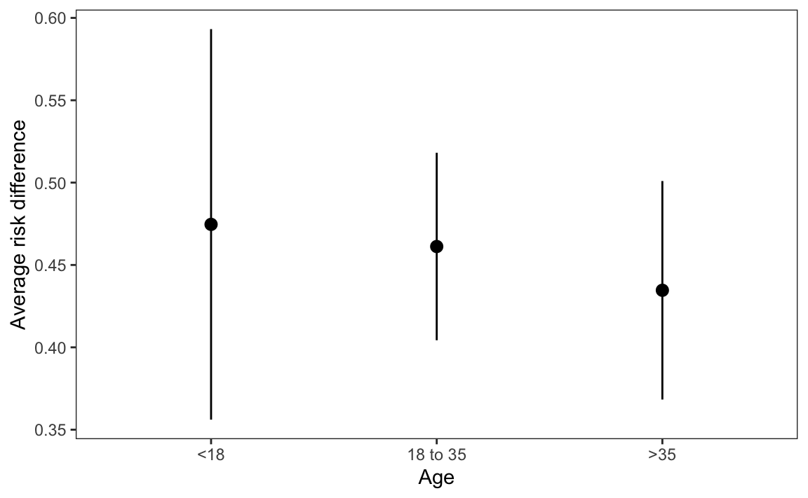
Figure 6.2: Marginal counterfactual comparisons for a change in incentive, by age category.
plot_comparisons(mod, variables ="incentive", by ="agecat").show()
This plot shows that, on average, our model expects that receiving an incentive will have a stronger effect on the probability of seeking to learn one’s HIV status for younger individuals. Indeed, the point estimate is higher on the left side of the plot than on the right side. However, the confidence intervals are wide and overlapping, which suggests that the treatment effects are not significantly different from one another.
6.6.2 Conditional comparisons
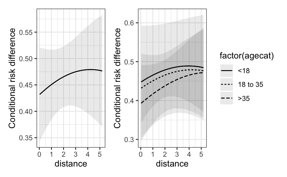
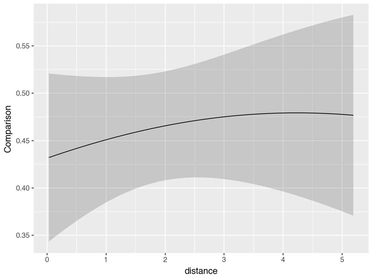
When one of the predictors of interest is continuous or when we are dealing with multiple predictors, plotting conditional comparisons rather than marginal ones can improve interpretability. The condition argument of the plot_comparisons() function helps us construct plots where we hold some predictors at representative values, while displaying the variation in comparisons for others.
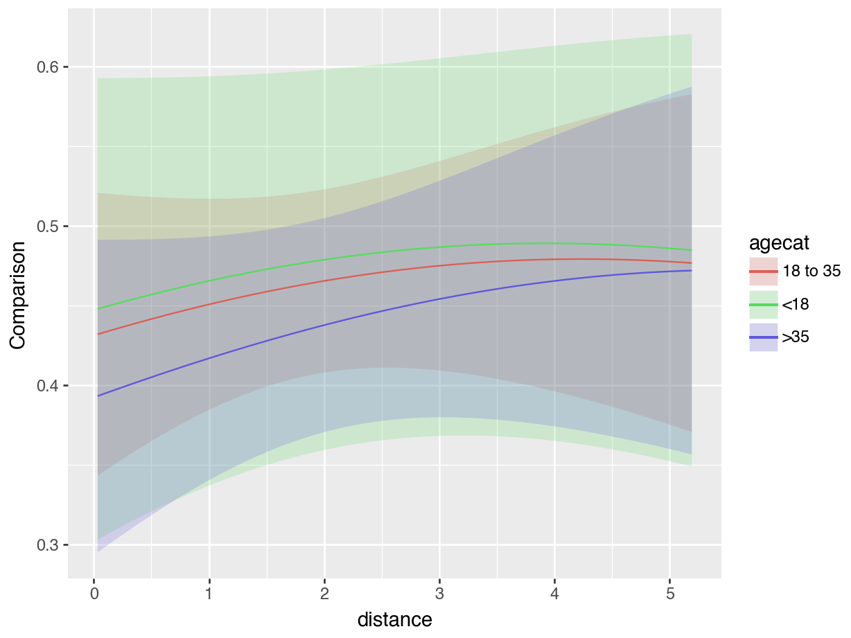
On these plots, high values on the y-axis indicate that the incentive has a strong effect on the predicted probability of outcome. The x-axis represents the distance between a participant’s home and the test center, with people living closest to the test center at the left of the plots.
The first plot shows that the estimated effect of incentive on the predicted probability of outcome is smaller for individuals living closest to the test center. The second plot further indicates slight differences across age groups, with older participants reacting less strongly to the treatment. Chapter 10 shows how to explore these kinds of contrasts more formally; it shows how to design and interpret tests of treatment effect heterogeneity, using interactions and polynomials.
6.7 Summary
This chapter defined a “counterfactual comparison” as a function of two or more model-based predictions made with different predictor values. These comparisons measure the strength of association between variables or, if appropriate identification assumptions are met, they quantify causal effects.
The comparisons() function from the marginaleffects package computes counterfactual comparisons for a wide range of models, and avg_comparisons() aggregates them across units or groups. Analysts can visualize these comparisons with the plot_comparisons() function or standard visualization tools like ggplot2.
Fitted model used to make counterfactual comparisons.
variables
Focal predictor whose association with or effect on the outcome we are interested in.
newdata
Grid of predictor values.
comparison
How the counterfactual predictions are compared: difference, ratio, lift, etc.
vcov
Standard errors: classical, robust, clustered, etc.
conf_level
Size of the confidence intervals.
type
Type of predictions to compare: response, link, etc.
cross
Estimate the effect of changing multiple variables at once (cross-contrast).
by
Grouping variable for average predictions.
wts
Weights used to compute average comparisons.
transform
Post-hoc transformations.
hypothesis
Compare different comparisons to one another, conduct linear or non-linear hypothesis tests, or specify null hypotheses.
equivalence
Equivalence tests
df
Degrees of freedom for hypothesis tests.
numderiv
Algorithm used to compute numerical derivatives.
...
Additional arguments are passed to the predict() method supplied by the modeling package.
To define, compute, and interpret counterfactual comparisons, analysts must make five decisions.
First, the Quantity:
Counterfactual comparisons are defined along two dimensions.
What change in focal predictor are we interested in? For example, do we want to estimate the effect of changing \(X\) from 0 to 1, of an increase of 1 unit or one standard deviation, or a change between two specific values. The change of focal predictor is specified by the variables argument.
What function do we use to compare counterfactual predictions? Two counterfactual predictions can be compared by a difference, ratio, lift, and many other functions. These comparisons are specified using the comparison argument in the comparisons() function.
Second, the Predictors:
Counterfactual comparisons are conditional quantities. They usually depend on the values of all predictors in a model.
Analysts can evaluate comparisons for different predictor grids, including empirical, balanced, interesting, or counterfactual grids, defined by the newdata argument and the datagrid() function.
Third, the Aggregation:
Analysts can report unit-level or aggregated counterfactual comparisons:
Unit-level comparisons: Specific to each observation.
Aggregated comparisons: Average effects or associations across the population or subgroups, computed with avg_comparisons() and the by argument.
Fourth, the Uncertainty:
The uncertainty around counterfactual comparisons can be estimated using classical or robust standard errors, bootstrap, or simulation-based inference.
Standard errors and confidence intervals are handled by the vcov and conf_level arguments, or via the inferences() function.
Fifth, the Test:
Hypothesis tests can check if counterfactual comparisons differ significantly from a null value or from one another. This is implemented with the hypothesis argument.
Equivalence tests can establish whether comparisons are practically equivalent to a reference value using the equivalence argument.
Goldsmith-Pinkham, Paul, Peter Hull, and Michal Kolesár. Forthcoming. “Contamination Bias in Linear Regressions.”American Economic Review, Forthcoming.
Horst, Allison Marie, Alison Presmanes Hill, and Kristen B Gorman. 2020. Palmerpenguins: Palmer Archipelago (Antarctica) Penguin Data. https://doi.org/10.5281/zenodo.3960218.
Thornton, Rebecca L. 2008. “The Demand for, and Impact of, Learning HIV Status.”American Economic Review 98 (5): 1829–63.
Westreich, Daniel, and Sander Greenland. 2013. “The Table 2 Fallacy: Presenting and Interpreting Confounder and Modifier Coefficients.”American Journal of Epidemiology 177 (4): 292–98. https://doi.org/10.1093/aje/kws412.
Zeileis, Achim, Susanne Köll, and Nathaniel Graham. 2020. “Various Versatile Variances: An Object-Oriented Implementation of Clustered Covariances in R.”Journal of Statistical Software 95 (1): 1–36. https://doi.org/10.18637/jss.v095.i01.
We take the log odds ratios of the averages, rather than the average log odds ratio, because odds ratios are non-collapsible.↩︎
Interpreting the parameters associated with adjustment variables as measures of association or effect is generally not recommended. See the discussion of Table 2 fallacy in Section 2.2 and Westreich and Greenland (2013).↩︎
See Section 2.1.3 for a discussion of the problems that can arise when multiple focal variables are included in a single model. Also see Goldsmith-Pinkham et al. (Forthcoming).↩︎
In the current example, computing the average across the full empirical distribution or in the subset of actually treated units does not make much difference, which is often the case for randomized controlled experiments. As Chapter 8 shows, this is not the case in general.↩︎
The statistic argument allows us to display confidence intervals instead of the default standard errors. The fmt determines the number of digits to display. gof_omit omits all goodness-of-fit statistics from the bottom of the table. shape indicates that models should be displayed as columns and terms and contrasts as structured rows.↩︎