            Estimate Std. Error t value Pr(>|t|)
(Intercept) -0.05033    0.09740  -0.517   0.6065
X            1.12963    0.09929  11.377   <0.001
Z 0.28486 0.11013 2.587 0.011214 Uncertainty
This chapter introduces four approaches to quantify uncertainty around quantities of interest: the delta method, bootstrap, simulation-based inference, and conformal prediction. We discuss the intuition behind each of these strategies, and reinforce that intuition by implementing simple versions “by hand.” The code examples are presented for pedagogical purposes; more robust and convenient implementations are supplied by the marginaleffects package. Readers who are not familiar with the basics of multivariable calculus may want to skip this chapter.
14.1 Delta method
The delta method is a statistical technique used to approximate the variance of a function of random variables. For example, data analysts often want to compare regression coefficients or predicted probabilities by subtracting them from one another. Such comparisons can be expressed as functions of a model’s parameters, but the variances (and standard errors) of such transformed quantities can be difficult to derive analytically. The delta method is a convenient way to approximate those variances. It allows us to quantify uncertainty around most of the quantities of interest discussed in this book.
The delta method is useful, versatile, and fast. Yet, the technique also has important limitations: it relies on a coarse linear approximation, its desirable properties depend on the asymptotic normality of the estimator,1 and it is only valid when a function is continuously differentiable in a neighborhood of its parameters. When analysts do not believe that these conditions hold, they can turn to the bootstrap or simulation-based inference.2
The theoretical properties of the delta method are discussed and proved in many textbooks (Wasserman 2004; Hansen 2022b; Berger and Casella 2024). Instead of demonstrating them anew, the rest of this section provides a hands-on tutorial, with a focus on computation. The goal is to reinforce intuitions by illustrating how to calculate standard errors manually in two cases: univariate and multivariate. Then, we briefly consider the use of robust or clustered standard errors.
14.1.1 Univariate delta method
In this section, we use the delta method to compute the standard error of a function with one parameter: the natural logarithm of a single regression coefficient. Consider a setting with three measured variables: \(Y\), \(X\), and \(Z\). With these variables in hand, the analyst estimates a linear regression model.
\[ Y = \beta_1 + \beta_2 X + \beta_3 Z + \varepsilon \tag{14.1}\]
Let \(\hat{\beta}_2\) be an estimator of the true parameter \(\beta_2\). We know that the variance of \(\hat{\beta}_2\) is \(\text{Var}(\hat{\beta}_2)\), but we are not interested in this particular statistic. Rather, our goal is to compute the variance of a function of the estimator: \(\text{Var}\left [\log(\hat{\beta}_2) \right ]\).
To get there, we apply a Taylor series expansion. This mathematical tool allows us to rewrite smooth functions like \(\log(\hat{\beta}_2)\) as infinite sums of derivatives and polynomials. This is a useful way to simplify and approximate complex functions.
The Taylor series of a function \(g(a)\) is always expressed by reference to a particular point \(\alpha\), where we wish to study the behavior of \(g\). Generically, the approximation can be written as
\[ g(a) = g(\alpha) + g'(\alpha)(a - \alpha) + \frac{g''(\alpha)}{2!}(a - \alpha)^2 + \cdots + \frac{g^{(n)}(\alpha)}{n!}(a - \alpha)^n + \cdots, \tag{14.2}\]
where \(g^{(n)}(\alpha)\) denotes the \(n\)th derivative of \(g(a)\), evaluated at \(a=\alpha\).
Equation 14.2 is an infinite series, so it is not practical (or possible) to compute all its terms. In real-world applications, we thus truncate the series by dropping higher-order terms. For instance, we can construct a first-order Taylor series by keeping only the first two terms on the right-hand side of Equation 14.2.
We can now approximate the function that interests us, \(\log(\hat{\beta}_2)\), as a first-order Taylor series, about the true value of the parameter \(\beta_2\). Recall that the derivative of \(\log(\beta_2)\) is \(1/\beta_2\), and substitute appropriate values into the first two terms of Equation 14.2.
\[\begin{align*} g(a) \approx g(\alpha) + g'(\alpha)(a - \alpha) \\ \log(\hat{\beta}_2) \approx \log(\beta_2) + \frac{1}{\beta_2}(\hat{\beta}_2 - \beta_2) \end{align*}\]
Now, insert the approximation in the variance operator.
\[ \text{Var}\left [\log(\hat{\beta}_2)\right ] \approx \text{Var} \left [\log(\beta_2) + \frac{1}{\beta_2}(\hat{\beta}_2 - \beta_2)\right ] \tag{14.3}\]
This linearized approximation of the variance is useful, because it allows further simplification. First, we know that the variance of a constant like \(\beta_2\) is zero, which means that some of the terms in Equation 14.3 can drop out. Second, we can apply the scaling property of variances3 to rewrite the expression as
\[ \text{Var}\left [\log(\hat{\beta}_2)\right ] \approx \frac{1}{\beta_2^2}\text{Var} \left [\hat{\beta}_2\right ] \tag{14.4}\]
Equation 14.4 gives us a formula to approximate the variance of \(\log(\hat{\beta}_2)\). This formula is expressed in terms of \(\text{Var}(\hat{\beta}_2)\), that is, the square of the estimated standard error. Equation 14.4 also includes the expression \(1/\beta_2\). Since we do not know the true value of that term, we fall back to using \(1/\hat{\beta}_2\) as a plug-in estimate.4
To show how this formula can be applied in practice, let’s simulate data that conform to Equation 14.1, and use that data to fit a linear regression model.
The true \(\beta_2\) is 1, but the estimated \(\hat{\beta}_2\) is
b2 = coef(mod)[2]
b2
[1] 1.129626The estimated variance of \(\hat{\beta}_2\) is
v = vcov(mod)[2, 2]
v
[1] 0.009859151The natural logarithm of our estimate, \(\log(\hat{\beta}_2)\), is
log(b2)[1] 0.1218865Using Equation 14.4, we compute the delta method estimate of \(\text{Var}\left [\log(\hat{\beta}_2)\right ]\), and we take its square root to obtain the standard error.
sqrt(v / b2^2)[1] 0.08789924To verify that this result is correct, we can use the hypotheses() function from the marginaleffects package. As noted in Chapter 4, hypotheses() can compute arbitrary functions of model parameters, along with standard errors.
library(marginaleffects)
hypotheses(mod, "log(b2) = 0")| Hypothesis | Estimate | Std. Error | z | Pr(>|z|) | 2.5 % | 97.5 % |
|---|---|---|---|---|---|---|
| log(b2)=0 | 0.122 | 0.0879 | 1.39 | 0.166 | -0.0504 | 0.294 |
Reassuringly, the estimate and standard error that we computed “manually” for \(\log(\hat{\beta}_2)\) are the same as the ones obtained “automatically” by calling hypotheses().
14.1.2 Multivariate delta method
The univariate version of the delta method can be generalized to the multivariate case. Let \(\mathcal{B}=\{\beta_1,\beta_2,\ldots,\beta_k\}\) be a vector of input parameters, and \(\Theta=\{\theta_1,\theta_2,\ldots,\theta_n\}\) represent the vector-valued output of an \(h\) transformation. For example, \(\mathcal{B}\) could be a vector of regression coefficients. \(\Theta\) could be a single summary statistic, or it could be a vector of length \(n\) with one fitted value per observation in the dataset.5
Our goal is to compute standard errors for each element of \(\Theta\). To do this, we express the multivariate delta method in matrix notation
\[ \operatorname{Var}\left(h(\mathcal{B})\right) = J^T \cdot \operatorname{Var}\left (\mathcal{B}\right ) \cdot J, \tag{14.5}\]
where \(h(\mathcal{B})\) is a function of the parameter vector \(\mathcal{B}\) and \(\text{Var}(h(\mathcal{B}))\) is the variance of that function.
\(J\) is the Jacobian of \(h\). The number of rows in that matrix is equal to the number of parameters in the input vector \(\mathcal{B}\). The number of columns in \(J\) is equal to the number of elements in the output vector \(\Theta\), that is, equal to the number of transformed quantities of interest that \(h\) produces. The element in the \(i\)th row and \(j\)th column of \(J\) is a derivative which characterizes the effect of a small change in \(\beta_i\) on the value of \(\theta_j\).
\[ J = \begin{bmatrix} \frac{\partial \theta_1}{\partial \beta_1} & \frac{\partial \theta_2}{\partial \beta_1} & \cdots & \frac{\partial \theta_n}{\partial \beta_1} \\ \frac{\partial \theta_1}{\partial \beta_2} & \frac{\partial \theta_2}{\partial \beta_2} & \cdots & \frac{\partial \theta_n}{\partial \beta_2} \\ \vdots & \vdots & \ddots & \vdots \\ \frac{\partial \theta_1}{\partial \beta_k} & \frac{\partial \theta_2}{\partial \beta_k} & \cdots & \frac{\partial \theta_n}{\partial \beta_k} \end{bmatrix} \]
Now, let’s go back to the linear model defined by Equation 14.1, with coefficients \(\beta_1\), \(\beta_2\), and \(\beta_3\). Imagine that we want to estimate the difference between the 2nd and 3rd coefficients of this model. This difference can be expressed as the single output \(\theta\) from a function \(h\) of three coefficients
\[ \theta = h(\beta_1,\beta_2,\beta_3) = \beta_2 - \beta_3, \tag{14.6}\]
or
b = coef(mod)
b[2] - b[3]
[1] 0.8447632To quantify the uncertainty around \(\theta\), we use the multivariate delta method formula. In Equation 14.5, \(\text{Var}(\mathcal{B})\) refers to the variance-covariance matrix of the regression coefficients, which we can extract using the vcov() function.
V = vcov(mod)
V
(Intercept) X Z
(Intercept) 0.0094869866 0.0009058965 0.0002349717
X 0.0009058965 0.0098591507 0.0005353338
Z 0.0002349717 0.0005353338 0.0121275336The \(J\) matrix is defined by reference to the \(h\) function. In Equation 14.6, \(h\) accepts three parameters as inputs and returns a single value. Therefore, the corresponding \(J\) matrix must have 3 rows and 1 column. We populate this matrix by taking partial derivatives of Equation 14.6 with respect to each of the input parameters.
\[ J = \left [ \begin{matrix} \frac{\partial \theta}{\beta_1} \\ \frac{\partial \theta}{\beta_2} \\ \frac{\partial \theta}{\beta_3} \end{matrix} \right ] = \left [ \begin{matrix} 0 \\ 1 \\ -1 \end{matrix} \right ] \]
Having extracted \(\text{Var}(\mathcal{B})\) and defined an appropriate \(J\) for the quantity of interest \(\theta\), we now use Equation 14.5 to compute the standard error.
[1] 0.1446237We have thus estimated that the difference between \(\beta_2\) and \(\beta_3\) is 0.845, and that the standard error associated with this difference is 0.145. Again, checking this result against the output of the hypotheses() function shows that they are identical.
hypotheses(mod, hypothesis = "b2 - b3 = 0")| Hypothesis | Estimate | Std. Error | z | Pr(>|z|) | 2.5 % | 97.5 % |
|---|---|---|---|---|---|---|
| b2-b3=0 | 0.845 | 0.145 | 5.84 | <0.001 | 0.561 | 1.13 |
14.1.3 Robust or clustered standard errors
The calculations in the previous sections relied on “classical” estimates of the variance-covariance matrix. These estimates are useful, but they rely on strong assumptions that rule out ubiquitous phenomena like autocorrelation, heteroskedasticity, and clustering.6 Where such patterns occur, classical standard errors may inaccurately characterize the uncertainty in our estimates.
To see how the assumptions that underpin classical standard errors can be relaxed, let’s consider a simple linear regression
\[ Y = X \beta + \varepsilon, \]
where \(Y\) is an \(n \times 1\) vector of outcome; \(X\) is an \(n \times k\) matrix of covariates, including an intercept; \(\beta\) is a \(k \times 1\) vector of coefficients; \(\varepsilon\) is an \(n \times 1\) vector of errors. We can estimate regression coefficients by ordinary least squares using the standard formula.
\[ \hat{\beta}=(X^TX)^{-1}(X^TY) \tag{14.7}\]
The usual way to compute the variance of \(\hat{\beta}\) in this context is to use the “sandwich” formula, so-called because it includes a “meat” expression, squeezed between identical “bread” components. The classical variance estimate for ordinary least squares can thus be written as
\[ Var(\hat{\beta}) = (X^TX)^{-1}(\sigma^2_\varepsilon X^TX)(X^TX)^{-1}, \tag{14.8}\]
where \(\sigma^2_\varepsilon\) can be estimated by taking the variance of estimated residuals.
To illustrate the use of these formulas, let’s load the Thornton (2008) data and fit a linear regression model with one predictor and an intercept.
library(sandwich)
library(marginaleffects)
dat = get_dataset("thornton")
dat = na.omit(dat[, c("incentive", "outcome")])
mod = lm(outcome ~ incentive, data = dat)
summary(mod)
Estimate Std. Error t value Pr(>|t|)
(Intercept) 0.33977 0.01695 20.04 <0.001
incentive 0.45106 0.01919 23.50 <0.001The same estimates can be obtained manually by constructing a design matrix \(X\), a response matrix \(Y\), and by applying Equation 14.7.
          [,1]
[1,] 0.3397746
[2,] 0.4510603
The variance-covariance matrix for these coefficients is obtained via Equation 14.8.
              [,1]          [,2]
[1,]  0.0002874265 -0.0002874265
[2,] -0.0002874265  0.0003684119
This is the same as the matrix returned by the vcov() function from base R.
vcov(mod) (Intercept) incentive
(Intercept) 0.0002874265 -0.0002874265
incentive -0.0002874265 0.0003684119And the square root of the diagonal elements of this matrix are the standard errors printed in the model summary at the top of this section.
One key assumption about classical standard errors is encoded explicitly in Equation 14.8. In that formula, and in the code that implements it, \(\sigma^2_\varepsilon\) is a single number, treated as a constant that reflects the uncertainty for each observation uniformly. But in many applied contexts, the variance in errors is not uniform, that is, there is heteroskedasticity.7
One popular strategy to overcome with this challenge is to report “robust” standard errors, also known as “heteroskedasticity-consistent” or “Huber-White” standard errors. There are many types of robust standard errors available, designed to address different data issues (Zeileis et al. 2020). The code below shows one of the simplest ways to account for heteroskedasticity. It implements the same sandwich formula as in the classical case, but the “meat” component includes a matrix with squared residuals on the diagonal. This gives us more flexibility to account for changes in the variance of prediction errors across the sample.
              [,1]          [,2]
[1,]  0.0003612364 -0.0003612364
[2,] -0.0003612364  0.0004362886
A more convenient way to compute the same variance-covariance matrix is to use the vcovHC() function from the powerful sandwich package, which supports many models and estimators beyond linear regression.
vcovHC(mod, type = "HC0") (Intercept) incentive
(Intercept) 0.0003612364 -0.0003612364
incentive -0.0003612364 0.0004362886In all marginaleffects functions, there is a vcov argument that allows us to report various types of robust standard errors. When that argument is omitted, marginaleffects returns estimates with classical standard errors. To report heteroskedasticity consistent standard errors instead, we simply add vcov. For example, the next line of code returns an estimate of the average counterfactual comparison (risk difference) with heteroskedasticity-consistent standard error.
avg_comparisons(mod, vcov = "HC0")| Estimate | Std. Error | z | Pr(>|z|) | 2.5 % | 97.5 % |
|---|---|---|---|---|---|
| 0.451 | 0.0209 | 21.6 | <0.001 | 0.41 | 0.492 |
The vcov argument accepts several string shortcuts like the one above. It can also take a variance-covariance matrix, a function that returns such a matrix, or a formula to specify clusters. The code block below shows a few examples, but readers are encouraged to consult the manual pages by typing ?hypotheses in R or help(hypotheses) in Python.
V = sandwich::vcovHC(mod)
avg_comparisons(mod, vcov = V)         # heteroskedasticity-consistent
avg_comparisons(mod, vcov = ~ village) # clustered by village
In sum, we have seen that the delta method is a simple, fast, and flexible approach to obtain standard errors for a vast array of quantities of interest. It is the default approach implemented by all the functions in the marginaleffects package. By combining the delta method with robust estimates of the variance-covariance matrix, analysts can report uncertainty estimates that account for common data features like heteroskedasticity or clustering.
14.2 Bootstrap
The bootstrap is a method pioneered by Bradley Efron and colleagues in the 1970s and 1980s (Efron and Tibshirani 1994). It is a powerful strategy to quantify uncertainty about quantities of interest.8
Consider \(T_n\), a statistic we wish to compute. \(T_n\) is a function of an outcome \(Y\), some regressors \(\mathbf{X}\), and the unknown population distribution function \(F\):
\[T_n = T_n ((Y_1,\mathbf{X}_1),\dots,(Y_n,\mathbf{X}_n),F)\]
The statistic of interest \(T_n\) follows a sampling distribution \(G\), which depends on the unknown population distribution \(F\). If we knew \(F\), then \(G\) would immediately follow. The key idea of the bootstrap is to use simulations to approximate \(F\), and then to use that approximation when quantifying uncertainty around the quantity of interest.
How do we approximate \(F\) in practice? Since the 1980s, many variations on bootstrap simulations have been proposed. A survey of this rich literature lies outside the scope of this book, but it is instructive to consider one of the simplest approaches: the non-parametric bootstrap algorithm. The idea is to build several simulated datasets by drawing repeatedly from the observed sample. With those datasets in hand, we can estimate the statistic of interest multiple times, and characterize its sampling distribution.
To illustrate, let’s consider a simple linear model fit to the Thornton (2008) data. The response is outcome, which is a binary variable equal to 1 for study participants who sought to learn their HIV status, and 0 for the others. There are three coefficients, each representing an age category.
dat = get_dataset("thornton")
mod = lm(outcome ~ agecat - 1, data = dat)
coef(mod)
agecat<18 agecat18 to 35 agecat>35
0.6718750 0.6787004 0.7277354 Our substantive goal is to determine if the proportion of individuals with outcome=1 is higher in the 35+ age group than in the 18-to-35 bracket. In other words, the quantity of interest is the difference between the 2nd and 3rd coefficients of the model. For convenience, we define a statistic() function to compute this difference.
[1] 0.04903501Now, let’s compute a bootstrap confidence interval around this quantity. This can be achieved in five steps:
- Sample rows with replacement from the original data.
- Fit the model to the new dataset.
- Compute the statistic using the new fitted model’s parameter estimates.
- Repeat steps 1 through 3 many times.
- Use quantiles of the bootstrap distribution to build a confidence interval around the statistic of interest.
The following code implements these five steps.
sample_fit_compute = function() {
  # Step 1: Sample
  index = sample(1:nrow(dat), size = nrow(dat), replace = TRUE)
  resample = dat[index, ]

  # Step 2: Fit
  mod_resample = lm(outcome ~ agecat - 1, data = resample)

  # Step 3: Compute
  statistic(mod_resample)
}

# Step 4: Repeat
set.seed(48103)
boot_dist = replicate(1000, sample_fit_compute())

# Step 5: Quantiles
ci = quantile(boot_dist, prob = c(0.025, 0.975))
ci
2.5% 97.5%
0.01435133 0.08701632 This analysis suggests that the estimated difference between the 3rd and the 2nd coefficient is 0.049, with a 95% confidence interval of [0.014, 0.087].
The inferences() function from marginaleffects makes this kind of analysis much easier, by providing a consistent interface to the boot, rsample, and fwb packages (Canty and Ripley 2022; Frick et al. 2022; Greifer 2022). This empowers users to apply a wide variety of bootstrap resampling schemes. To use this functionality, we call any of the core marginaleffects functions, and pass its output to inferences().9
hypotheses(mod, "b3 - b2 = 0") |>
inferences(method = "boot", R = 1000)| Hypothesis | Estimate | 2.5 % | 97.5 % |
|---|---|---|---|
| b3-b2=0 | 0.049 | 0.0156 | 0.0846 |
The results are close those obtained manually, but they vary a little bit due to the random nature of the procedure and minor differences in the resampling scheme.
Note that the same workflow works for other marginaleffects functions, such as avg_comparisons().
avg_comparisons(mod) |> inferences(method = "boot")| Contrast | Estimate | 2.5 % | 97.5 % |
|---|---|---|---|
| 18 to 35 - <18 | 0.00683 | -0.05439 | 0.0668 |
| >35 - <18 | 0.05586 | -0.00393 | 0.1158 |
Bootstrapping is a versatile approach to estimate the sampling distribution of a statistic. It is widely applicable, even if we do not know the underlying distribution of the quantities of interest, making it a powerful tool for deriving standard errors and confidence intervals. However, bootstrapping can be computationally intensive, particularly for large datasets or complex models. In addition, selecting an adequate resampling scheme can be challenging when the data-generating process is complex.
14.3 Simulation
Yet another strategy to estimate the uncertainty around quantities of interest is simulation-based inference. This method is an alternative to traditional analytical approaches, leveraging the power of computational simulations to estimate the variability of a given function of parameters. One of the earliest applications of this approach can be found in Krinsky and Robb (1986), who use simulations to quantify the sampling uncertainty around estimates of elasticities in a regression modeling context. King et al. (2000) subsequently popularized the strategy and its implementation in the clarify software.10
The foundational assumption of this approach is that a regression-based estimator is normal. This allows us to leverage the properties of the multivariate normal distribution to simulate many sets of coefficients, and many quantities of interest. This can be done in 3 steps:
- Draw many sets of parameters from a multivariate normal distribution, with mean equal to the estimated vector of coefficients, and variance equal to the estimated covariance matrix.
- Compute the statistic using each set of simulated coefficients.
- Build a confidence interval for the quantity of interest by taking quantiles of the simulated quantities.
As Rainey (2024) notes, this process can be thought of as an informal Bayesian posterior simulation. While it does not strictly use Bayesian methods, it shares a similar outlook, using the distribution of simulated parameters to infer the uncertainty around transformed quantities. By repeatedly sampling from the parameter space, we can gain a clearer picture of the possible variability.
The code below implements a simple version of this strategy.
# Step 1: Simulate coefficients
library(mvtnorm)
set.seed(48103)
coef_sim = rmvnorm(1000, coef(mod), vcov(mod))

# Step 2: Compute the quantity of interest
statistics = coef_sim[, 3] - coef_sim[, 2]

# Step 3: Build confidence intervals as quantiles
ci = quantile(statistics, probs = c(0.025, 0.975))
ci
2.5% 97.5%
0.01343765 0.08461654 Note that the simulation-based confidence interval is slightly different from those obtained via bootstrap or delta method, but it has the same general magnitude.
We can obtain similar results with the inferences() function.
hypotheses(mod, "b3 - b2 = 0") |>
inferences(method = "simulation", R = 1000)| Hypothesis | Estimate | 2.5 % | 97.5 % |
|---|---|---|---|
| b3-b2=0 | 0.049 | 0.015 | 0.0871 |
avg_comparisons(mod, variables = "agecat") |>
inferences(method = "simulation", R = 1000)| Contrast | Estimate | 2.5 % | 97.5 % |
|---|---|---|---|
| 18 to 35 - <18 | 0.00683 | -0.05375 | 0.0607 |
| >35 - <18 | 0.05586 | -0.00286 | 0.1148 |
Simulation-based inference is easy to implement, convenient, and it applies to a broad range of models. It trades the analytic approximation of the delta method for a numerical approximation through simulation. Although simulation-based inference can be more computationally expensive than the delta method, it is usually faster than bootstrapping, which requires refitting the model multiple times.
14.4 Conformal prediction
In Chapter 5, we used the predictions() function to compute confidence intervals around fitted values. These intervals are designed to characterize the uncertainty about the model-based expected value of the response.
One common misunderstanding is that these confidence intervals should be calibrated to cover a certain percentage of unseen data points. This is not the case. In fact, a confidence interval built using the delta method will typically cover a much smaller share of out-of-sample observations than its nominal size would suggest.
To see this, let’s conduct a simulation with two samples of 25 observations drawn randomly from a normal distribution with mean \(\pi\). The \(Y_{train}\) set is used to fit a model, and the set \(Y_{test}\) is used to check the accuracy of the model’s predictions. The model we fit is a linear regression with only an intercept, and we use the predictions() function to compute a 90% confidence interval around the expected value of the response. Finally, we check how many observations in the test set are covered by this interval.
simulation = function(...) {
  # Draw random training and test sets
  Y_train = rnorm(25, mean = 3.141593)
  Y_test = rnorm(25, mean = 3.141593)

  # Fit an intercept-only linear model
  m = lm(Y_train ~ 1)

  # Predictions with 90% confidence interval
  p = predictions(m, conf_level = .90)

  # Does the confidence interval cover the true mean?
  coverage_mean = mean(p$conf.low < 3.141593 & p$conf.high > 3.141593)

  # Does the confidence interval cover out of sample observations?
  coverage_test = mean(p$conf.low < Y_test & p$conf.high > Y_test)

  out = c(
    "Mean coverage" = coverage_mean,
    "Out-of-sample coverage" = coverage_test)
  return(out)
}
To draw an overall portrait of performance, we repeat this experiment 1000 times, and report the average coverage across experiments.
         Mean coverage Out-of-sample coverage
               0.88100                0.24668
The confidence intervals produced by predictions() cover the true mean of the outcome nearly 90% of the time, which matches the significance level that we requested using the conf_level argument. However, the confidence intervals only cover out-of-sample observations 25% of the time. Clearly, if we want an interval to cover a pre-specified share of unseen data points, we cannot rely on confidence intervals. We must compute prediction intervals instead.
How can we obtain prediction intervals with adequate coverage? In their excellent tutorial, Angelopoulos and Bates (2022) introduce “conformal prediction” as
“a user-friendly paradigm for creating statistically rigorous uncertainty sets/intervals for the predictions of such models. Critically, the sets are valid in a distribution-free sense: they possess explicit, non-asymptotic guarantees even without distributional assumptions or model assumptions.”
These are extraordinary claims which deserve to be repeated and emphasized. Conformal prediction can offer well-calibrated intervals, that cover a known share of out-of-sample data points, in finite samples, without making distributional assumptions, and even if the prediction model is misspecified.
There are three main caveats to this. First, the conformal prediction algorithms implemented in marginaleffects are designed for exchangeable data.11 They do not offer coverage guarantees in contexts where exchangeability is violated, such as in time series data, when there is spatial dependence between observations, or when there is distribution drift between the training and test data. Second, these algorithms offer marginal coverage guarantees, that is, they guarantee that a random test point will fall within the interval with a given probability. Such intervals may not be well calibrated locally, in different strata of the predictors.12 Third, the width of the conformal prediction interval will typically depend on the quality of the prediction model and of the function that we use to characterize the “quality” of predictions (i.e., the “score” function).13
A detailed technical treatment of conformal prediction lies outside the scope of this book, but we can form some intuition by considering two prediction tasks: numeric and categorical outcomes.
14.4.1 Numeric outcome
This introduction to conformal prediction adopts a code-first rather than a theory-heavy approach. To make things concrete, we will consider a dataset which contains demographic information on over 1 million members of the US military, including variables such as grade, branch, gender, race, and rank. Our prediction task involves using a linear model to predict the rank of military personnel based on these individuals’ characteristics.
library(marginaleffects)
dat = get_dataset("military")
head(dat)
rownames grade branch gender race hisp rank officer
1 1 officer army male ami/aln TRUE 2 1
2 2 officer army male ami/aln TRUE 2 1
3 3 officer army male ami/aln TRUE 5 1
4 4 officer army male ami/aln TRUE 5 1
5 5 officer army male ami/aln TRUE 5 1
6 6 officer army male ami/aln TRUE 5 1There are many algorithms available to build prediction intervals. For illustration, we will use one of the simplest: split conformal prediction. The first step of this strategy is to split the dataset randomly into three parts.14 The training set is used to fit the prediction model. The calibration set is used by the conformal prediction algorithm to determine the appropriate width of prediction intervals. The test set is used to evaluate the accuracy of out-of-sample predictions.
Now we use the training data to fit a linear regression model. Our goal is to predict the rank of an individual member of the military, based on four predictors.
                      Estimate Std. Error  t value Pr(>|t|)
(Intercept)           5.900195   0.020494  287.893   <0.001
gradeofficer         -1.288080   0.006967 -184.880   <0.001
gradewarrant officer -2.167464   0.021205 -102.213   <0.001
brancharmy           -0.192071   0.006500  -29.551   <0.001
branchmarine corps   -0.705205   0.008311  -84.848   <0.001
branchnavy           -0.064200   0.007314   -8.777   <0.001
gendermale            0.286665   0.007123   40.243   <0.001
raceasian             0.430081   0.022936   18.751   <0.001
raceblack             0.652504   0.019943   32.718   <0.001
racemulti            -0.584264   0.026247  -22.260   <0.001
racep/i              -0.025871   0.036875   -0.702    0.483
raceunk               1.261640   0.022067   57.173   <0.001
racewhite             0.401818   0.019304   20.816   <0.001
Split conformal inference leverages the assumption that observations in the calibration set are exchangeable for those in the test set. If, in that sense, the calibration set is similar to the test set, then it seems reasonable to expect that the prediction errors we make in one will be similar to the prediction errors we make in the other.15 With that in mind, we can study the calibration set to get a sense of how wide the prediction intervals should be.
The code below does three things: (1) use the fitted linear model to make predictions in the calibration set, (2) compute absolute residuals for each observation in the calibration set, and (3) plot the distribution of those residuals. The vertical dashed line shows the 95th quantile of absolute residuals.
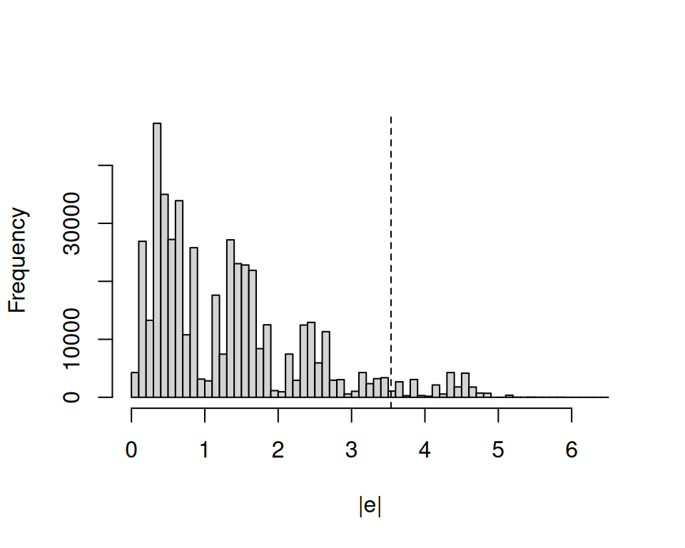
If the calibration and test sets are exchangeable, then it feels reasonable to expect that 95% of the absolute prediction errors that our model will make in the test set will fall to the left of the dashed line in Figure 14.1. Thus, if we want to construct a prediction interval that covers at least 95% of the points in the test set, we can define a constant \(d\) equal to the smallest absolute residual above the 95th percentile, and build prediction intervals as \(\hat{Y}_i\pm d\).
Finally, we can check how many of the unseen data points in the test set are covered by the split conformal prediction sets.
covered = dat$test$rank > conformal_lo & dat$test$rank < conformal_hi
mean(covered)
[1] 0.9515136We find that 95.2% of observations in the test set are covered. This is very close to our target coverage rate of 95%.
Instead of doing all that by hand, we can use the inferences() function from the marginaleffects package, which yields identical results.
p = predictions(mod) |>
  inferences(
    method = "conformal_split",
    conformal_calibration = dat$calib,
    conformal_test = dat$test)

covered = p$rank > p$pred.low & p$rank < p$pred.high
mean(covered)
[1] 0.951513614.4.2 Categorical outcome
Now, let’s illustrate an analogous strategy in the context of a classification task. We use a multinomial logit model to predict what branch of the military each observation belongs to: air force, army, marine corps, or navy.
The key difference with the previous section is that the outcome is now nominal, rather than numeric. For each observation in the test set, we want to predict a set of classes that should include the true value with a specified probability. For some individual, the model could thus predict a set of classes {navy, air force} that, we hope, includes the true branch to which the individual belongs.
Recall that conformal prediction requires us to quantify the quality of predictions in a calibration dataset. Instead of using a residuals-based approach as in the previous section, we measure the quality of class predictions using a “softmax score,” derived from the probability that the model assigns to the true (observed) class. Also, rather than preparing a held-out calibration set as in Section 14.4.1, we use an alternative conformal algorithm based on cross-validation.16 These changes can be made easily by modifying the arguments of the inferences() function.
set.seed(48103)
p = predictions(mod, conf_level = .8) |>
    inferences(
        R = 5,
        method = "conformal_cv+",
        conformal_score = "softmax",
        conformal_test = dat$test)
The inferences() returns a data frame with one row per observation in the test set. The pred.set column from that data frame includes one list of possible classes, for each observation.
Consider the last individual in our test set. If we call predictions() on the data for that individual, we find that the most likely branch value “army.”
| Group | Estimate | Std. Error | z | Pr(>|z|) | 2.5 % | 97.5 % |
|---|---|---|---|---|---|---|
| air force | 0.365 | 0.00746 | 48.9 | <0.001 | 0.3503 | 0.380 |
| army | 0.422 | 0.00765 | 55.2 | <0.001 | 0.4073 | 0.437 |
| marine corps | 0.100 | 0.00466 | 21.6 | <0.001 | 0.0912 | 0.109 |
| navy | 0.112 | 0.00489 | 23.0 | <0.001 | 0.1028 | 0.122 |
predictions(mod, newdata = tail(dat$test, 1))However, making that single point prediction would be misleading, because that individual actually belongs to a different branch.
tail(dat$test$branch, 1)[1] "air force"Thankfully, our conformal prediction set included more than just a point prediction. Indeed, we see that the prediction set associated to that individual includes the most likely (but incorrect) branch, but also the correct result.
tail(p, 1)| Pred Set 97.5 % |
|---|
| air force, army |
More generally, we can check if the individual prediction sets include the true values of branch in the test set, using the code below.
As expected, conformal prediction sets include the correct value of about 80% of the time.
In conclusion, this chapter has explored various methods to quantify uncertainty in statistical analysis, including the delta method, bootstrap, simulation-based inference, and conformal prediction. Each method offers unique advantages and is suitable for different scenarios, depending on the assumptions one is willing to make and on the computational resources available. The delta method provides fast results using linear approximations, while the bootstrap and simulation-based inference leverage computational power to draw from re-sampled or simulated results. Conformal prediction offers distribution-free prediction intervals which, under certain conditions, can be expected to cover a specified share of unseen data points. Understanding these methods equips analysts with a comprehensive toolkit to address uncertainty in their analyses.
The delta method relies on the observation that if the distribution of a parameter is asymptotically normal, then the limiting distribution of a smooth function of this parameter is also normal (Wasserman 2004).↩︎
Let \(c\) be a constant and \(\lambda\) be a random variable, then \(\text{Var}[c\lambda]=c^2\text{Var}[\lambda]\).↩︎
Autocorrelation is often an issue in time series estimation when the prediction errors we make for a unit of observation at time \(t\) are correlated to the prediction errors we make for the same unit at time \(t+1\). Clustering sometimes occurs when errors are similar for study participants drawn from well-defined groups (e.g., classrooms, neighborhoods, or provinces). Heteroskedasticity arises when the variance of the errors is inconsistent across observations, such as when our model makes bigger prediction errors for units with certain characteristics. ↩︎
Footnote \(\ref{ft-heteroskedasticity}\)↩︎
The notation and ideas in this section follow Hansen (2022a).↩︎
Additional arguments can be passed to control functions from the bootstrap packages, by directly inserting them in the
inferences()call. See?boot::boot,?rsample::rsample, and?fwb::fwb↩︎clarifyis now available forR(Greifer et al. 2023).↩︎The usual “independent and identically distributed” assumption is a more restrictive special case of exchangeability.↩︎
Different algorithms have recently been proposed to offer class-conditional coverage guarantees (Ding et al. 2023). These algorithms are not currently implemented in
marginaleffects, but they are on the software development roadmap.↩︎Note that the score functions implemented in
marginaleffectssimply take the residual—or difference between the observed outcome and predicted value. This means that thetypeargument must ensure that observations and predictions are on commensurable scales (usuallytype="response"ortype="prob").↩︎In this case, the three datasets have approximately the same number of rows, but this need not be the case.↩︎
Prediction errors in the training set are usually smaller than errors in either the calibration or test sets, because of overfitting.↩︎
The split conformal algorithm would also work in this context. We use cross-validation simply for illustration.↩︎