2 Models and meaning
The best way to start a data analysis project is to set clear goals. This chapter explores four of the main objectives that data analysts pursue when they fit statistical models or deploy machine learning algorithms: model description, data description, causal inference, and out-of-sample prediction.
To achieve these goals, it is crucial to articulate well-defined research questions, and to explicitly specify the statistical quantities—the estimands—that can shed light on those questions. Ideally, estimands should be expressed in the simplest form possible, on a scale that feels intuitive to stakeholders, colleagues, and domain experts.
This chapter concludes by discussing some of the challenges that arise when trying to make sense of complex models. In many cases, the parameters of our models do not directly align with the estimands that actually interest us. Often, we must transform parameter estimates into quantities that directly inform our research questions, and that our audience will readily understand.
2.1 Why fit a model?
The first challenge that all researchers must take on is to transparently state what they hope to achieve with an analysis. Below, I survey four of the goals that an analyst can pursue: model description, data description, causal inference, and out-of-sample prediction.
2.1.1 Model description
The primary aim of model description is to understand how a fitted model behaves in different scenarios. Here, the focus is on the internal workings of the model itself, rather than on making predictions or inferences about the sample or population. The analyst peeks inside the “black-box” to audit, debug, or test how the model reacts to different inputs.
Model description aligns closely with the concepts of interpretability, explainability, and transparency in machine learning. It is an important activity, as it can provide some measure of reassurance that a fitted model works as intended, and is suitable for deployment.
To describe a fitted model’s behavior, the analyst might compute model-based predictions, that is, the expected value of the outcome variable for different subgroups of the sample.1 For example, a real estate analyst may check if their fitted model yields reasonable expectations about home prices in different markets, and go back to the drawing board if those expectations are unrealistic.
In a different context, the analyst may conduct a counterfactual analysis to see how a model’s predictions change when we alter the values of some predictors.2 For instance, a financial analyst may wish to guard against algorithmic discrimination by comparing what their model says about the default risk of borrowers from different ethnic backgrounds, when we hold other predictors constant.
2.1.2 Data description
Data description involves using statistical or machine learning models as tools to describe a sample, or to draw descriptive inference about a population. The objective here is to explore and understand the characteristics of the data, often by summarizing their (potentially joint) distribution. Descriptive and exploratory data analysis can help analysts uncover new patterns, trends, and relationships. It can stimulate the development of theory or raise new research questions (Tukey 1977).
Data description is arguably more demanding than model description, because it imposes additional assumptions. Indeed, if the sample used to fit a model is not representative of the target population, or if the estimator is biased, descriptive inference may be misleading.
To describe their data, an analyst might use a statistical model to compute the expected value of an outcome for different subgroups of the data.3 For example, a researcher could offer a summary description of forest coverage in the Côte Nord or Cantons de l’Est regions of Québec.
2.1.3 Causal inference
In causal inference our goal is to estimate the effect of an intervention (a.k.a., treatment, explanator, independent variable, or predictor) on some outcome (a.k.a., response or dependent variable). This is a fundamental activity in all fields where understanding the consequences of a phenomenon helps us make informed decisions or policy recommendations.
Causal inference is one of the most ambitious and challenging tasks in data analysis. It typically requires careful experimental design or statistical models that can adjust for all confounders in observational data. Several theoretical frameworks have been developed to help us understand the assumptions required to make credible claims about causality. Here, I briefly highlight two of the most important.
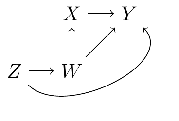
The structural causal models approach, developed by Judea Pearl and colleagues, encodes causal relationships as a set of equations that describe how variables influence each other. These equations can be represented visually by a directed acyclic graph (DAG), where nodes correspond to variables and arrows to causal effects. Consider Figure 2.1, which shows the causal relationships between a treatment \(X\), an outcome \(Y\), and two confounding variables \(Z\) and \(W\). Graphs like this one help us visualize the theorized data generating process and communicate our assumptions transparently. By analyzing a DAG, we can also learn if a research design and statistical model fulfill the conditions required to identify a causal effect in a given context.4
Another influential theoretical approach to causality is the potential outcomes framework, or Neyman-Rubin Causal Model. In this tradition, we think of causal effects as comparisons between potential outcomes: what would happen to the same individual under different treatment conditions? For each observation in a study, there are two potential outcomes. First, we ask what would happen if unit \(i\) received the treatment. Then, we ask what would happen if unit \(i\) did not receive the treatment. Finally, we define the causal effect as the difference between those two potential outcomes. Unfortunately, we can only observe one potential outcome at a time, because an individual cannot be part of both the treatment and control groups simultaneously. As a result, it is impossible to directly observe the effect of a treatment on any single unit of observation.5 This inconvenient fact is often dubbed the “fundamental problem of causal inference,” and it motivates the development of procedures to estimate aggregated or average treatment effects (see Chapters 6 and 8) .
The literature on causality is vast, and a thorough discussion of Structural Causal Models or the Neyman-Rubin Model lies outside the scope of this book.6 Nevertheless, it is useful to reflect a bit on the language that data analysts use when discussing their empirical results.
When a research design does not satisfy the strict requirements for causal identification, researchers will often revise their texts, replacing strong causal words by weak associational terms. For instance, they may strike out words like “cause”, “affect”, “influence”, or “increase” from observational studies, and replace them by terms such as “link”, “association”, or “correlation.” Paying attention to the words we use to describe statistical results is one way to remind our audience that association does not necessarily imply causation (Hill et al. 2024).
In recent years, though, some have started to push back against the use of causal euphemisms (Grosz et al. 2020; Hernán 2018). The problem is that researchers and their audiences often care about causation, not mere association, and that pretending otherwise may be counterproductive. Consider the large number of studies published on the “association between daily alcohol intake and risk of all-cause mortality” (Zhao et al. 2023). The research question that motivates this work is fundamentally causal: readers hope to learn how much longer they might live if they stopped drinking, and policy makers wish to know if discouraging alcohol intake would be good for public health. We do not care about mere association; we care about the effects of a cause!
Changing a few adjectives in a paper does not fundamentally change the research question, and it does not absolve us of the responsibility to justify our assumptions. In fact, avoiding causal language may introduce ambiguity about a researcher’s goals, and could hinder scientific progress.
What are we to do? One way out of this conundrum is transparency. Researchers can candidly state: “I am interested in the causal effect of \(X\) on \(Y\), but my research design and data are limited, so I cannot make strong causal claims.” When both the goals of an analysis and the violations of its assumptions are laid out clearly, readers can interpret (and discount) the results appropriately.
Part II of this book presents two broad classes of estimands which can be used to characterize either the “association” between two variables, or the “effect” of one variable on another (Chapters 6 and 7). When describing those quantities, I will not shy away from using causal words like “increase,” “change,” or “affect.” However, analysts should be mindful that when conditions for causal identification are violated, they have a duty to signal those violations explicitly and clearly to their audience.
2.1.4 Out-of-sample prediction
Out-of-sample prediction and forecasting aim to predict future or unseen data points based on a model fit on existing data. This is particularly challenging due to the need to ensure that our model does not overfit the data and generalizes well (James et al. 2021). Furthermore, out-of-sample prediction imposes additional requirements on the stability of the data distribution, and on the absence of changes in exogenous factors between the training sample and the target data. For example, a model trained to predict the probability of loan default may no longer perform well after an economic crisis changes the personal finances of a large portion of the population.
Out-of-sample prediction is not the main focus of this book, but Section 14.4 presents a case study on conformal prediction, a flexible strategy to make predictions and build intervals that will cover a specified proportion of out-of-sample observations.
2.2 What is your estimand?
Once the overarching goal of an analysis is posed, the next step is to rigorously define the target of our inquiry, that is, the specific value that would shed light on our research question. In this book, I will call this target the “quantity of interest” or the “estimand.”
An estimand is the quantity or parameter that we seek to learn. An estimator is the statistical method, algorithm, or mathematical formula that we apply to our data to gain insight into the estimand. An estimate is the numerical result that we obtain by applying an estimator to data; it is our best guess of the estimand’s true value based on the available information. For example, if we want to know the average height of all adults in a country (estimand), we might use the mean formula (estimator) to calculate that the average height is 170cm in a random sample from the population (estimate).
In statistical training and practice, much emphasis is placed on the various estimators that one can deploy, and on the interpretation of parameter estimates. Estimands do not always get as much attention. This is unfortunate, because a clear definition of the quantity of interest is essential to ensure that the estimator we choose, and the estimates we compute, speak to our research question. As Lundberg et al. (2021) write:
“In every quantitative paper we read, every quantitative talk we attend, and every quantitative article we write, we should all ask one question: what is the estimand? The estimand is the object of inquiry—it is the precise quantity about which we marshal data to draw an inference.”
This injunction is sensible, yet many of us conduct statistical tests without explicitly defining the quantity of interest, and without explaining exactly how this quantity answers the research question. This lack of clarity impedes communication between researchers and audiences, and it can lead us all astray.
To see how, imagine a dataset produced by the same data generating process as in Figure 2.1. Further assume that relationships between all variables are linear. In that context, we can estimate the causal effect of \(X\) and \(Y\) by fitting a linear model.7
\[ \text{Y} = \beta_1 + \beta_2 X + \beta_3 Z + \beta_4 W + \varepsilon \tag{2.1}\]
At first glance, it may seem that this model allows us to simultaneously and separately estimate the effects of \(X\), \(Z\), and \(W\) on \(Y\). Unfortunately, the coefficients in Equation 2.1 do not have such a straightforward causal interpretation.
On the one hand, the model includes enough control variables to eliminate confounding with respect to \(X\).8 As a result, \(\hat{\beta}_2\) can be interpreted causally, as an estimate of the effect of \(X\) on \(Y\). On the other hand, Equation 2.1 includes a control variable that is post-treatment with respect to \(Z\): the model adjusts for \(W\), which lies downstream on the causal path from \(Z\) and \(Y\). As a result, \(\hat{\beta}_3\) should not be interpreted as capturing the total causal effect of \(Z\) on \(Y\) (Keele et al. 2020; Cinelli et al. 2024).9
This illustrates what Westreich and Greenland (2013) call the “Table 2 Fallacy”: two similar-looking statistical quantities, estimated by a single regression model, can have very different substantive interpretations. More often than not, the coefficients associated with control variables in a regression model are incidental to the analysis. It is a mistake to interpret them individually, one after the other, as if they each captured a causal effect or correlation of interest. To avoid this trap, researchers must define their estimand explicitly, and only highlight the empirical quantities that are actually relevant to this estimand.
If defining one’s estimands is so important, why do many researchers neglect to do so? Part of the explanation may simply be that statistical and causal inference are hard problems. It can often be difficult for researchers to follow a consistent thread through theory development, study design, measurement, and statistical modeling, all the way to estimates. To compound this challenge, the terminology used to describe quantities of interest is, frankly, a big mess. In fact, many widely used technical terms have parallel or outright contradictory meanings.
Consider the popular expression “marginal effect.” In some disciplines, like economics and political science, a marginal effect is defined as the slope of the outcome with respect to one of the model’s predictors. In that context, the word “marginal” evokes the effect of a small change in one of the model’s predictors on the outcome.10 In contrast, researchers from other disciplines who write the same words usually signal that they are “marginalizing,” or taking an average of unit-level estimates.11 In the former case, “marginal effect” refers to a derivative; in the latter, it refers an integral. The same expression has two exactly opposite meanings!
One of the main goals of this book is to empower researchers to overcome terminological ambiguity, and to help them define estimands clearly and easily. To that end, Chapter 3 introduces a powerful new conceptual framework. By answering five simple questions, analysts can rigorously define their quantities of interest, and communicate their results clearly.
2.3 Making sense of parameter estimates
Consider a typical statistical setting where the analyst asks a research question and selects a model to meet domain-specific requirements. Perhaps the model is designed to capture a salient feature of the data-generating process, achieve a satisfactory level of goodness-of-fit, or control for confounders that could introduce bias in a causal estimate. The analyst fits their model using an estimator, and obtains parameter estimates along with standard errors.
Even if a fitted model is relatively simple, the parameter estimates it generates may not map directly onto an estimand that could inform one’s research question; the raw parameters may be very difficult to interpret substantively. For example, an analyst who fits a logistic regression model to a binary outcome will typically get coefficient estimates expressed as log odds ratios, that is, as the natural logarithm of a ratio-of-ratios-of-probabilities. Despite the simple nature of this model, its parameters are still expressed as complicated functions of probabilities.
But even the most straightforward probabilities are notoriously challenging to grasp intuitively. Indeed, a substantial body of literature in psychology and behavioral economics documents various biases that distort how individuals perceive and make decisions based on them. In their seminal work, Kahneman and Tversky (1979) argue that people tend to “underweight outcomes that are merely probable in comparison with outcomes that are obtained with certainty.” Numerous other biases have been identified over the years, including the “base rate fallacy” and various “conservative biases” (Nickerson 2004).
If understanding simple probabilities is already difficult, how can we expect colleagues and stakeholders to grasp weird concepts like odds ratios? How should we interpret the estimates produced by fancy regression models with splines and interactions? How can we help our audience understand the results produced by mixed-effects Bayesian models, or by complex machine learning algorithms?
The main contention of this book is that, in most cases, analysts should not focus on the raw parameters of their models. Instead, they should transform those parameters into quantities that make more intuitive sense, and that shed light directly onto their research question. Instead of reporting log odds ratios, analysts who fit logistic regressions should transform coefficients into predicted probabilities, and compare predictions made with different values of the predictors.
In Chapter 3, I will argue that this particular transformation, from logit coefficients to predicted probabilities, is but one example of a much more general workflow. This workflow can be applied consistently, in model-agnostic fashion, to interpret the results of over 100 different classes of statistical and machine learning models. By learning one conceptual framework, and one set of tools, analysts can make sense of an extraordinarily large array of modeling contexts.
One way to buttress claims of causal identification is to argue that a model satisfies the “backdoor criterion” (Pearl 2009). A set of control variables \(\mathbf{K}\) fulfills this criterion relative to a pair of variables \((X,Y)\) if no node in \(\mathbf{K}\) is downstream in the causal path from the treatment \(X\); and if elements of \(\mathbf{K}\) “block” every path between \(X\) and \(Y\) that contains an arrow into \(X\).↩︎
Note that repeated measurements do not solve this problem, since a person is not exactly identical at times \(t\) and \(t+1\).↩︎
Readers who need to know if their statistical results can be interpreted as causal estimates are encouraged to read one of the many excellent books published on the topic, e.g. Pearl (2009), Angrist and Pischke (2009), Morgan and Winship (2015), Imbens and Rubin (2015), Pearl and Mackenzie (2018), Hernán and Robins (2020), or Ding (2024).↩︎
If the DAG is correct, adjusting for \(W\) in the regression model is sufficient to satisfy the backdoor criterion (Hernán and Robins 2020). Controlling for \(Z\) is not strictly necessary to estimate the effect \(X\) on \(Y\), but it may improve the precision of our estimates.↩︎
In the language of Pearl and Mackenzie (2018) and Morgan and Winship (2015), the backdoors between \(X\) and \(Y\) are closed.↩︎
In the spirit of mediation analysis, \(\hat{\beta}_3\) could be interpreted as an estimate of the “direct” effect of \(Z\) on \(Y\), rather than its “total” effect. However, this interpretation requires stringent assumptions that are rarely satisfied in practice (Imai et al. 2011; Pearl 2014). Likewise, \(\hat{\beta}_4\) cannot be interpreted as the total effect of \(W\) on \(Y\).↩︎