11 Categorical and ordinal outcomes

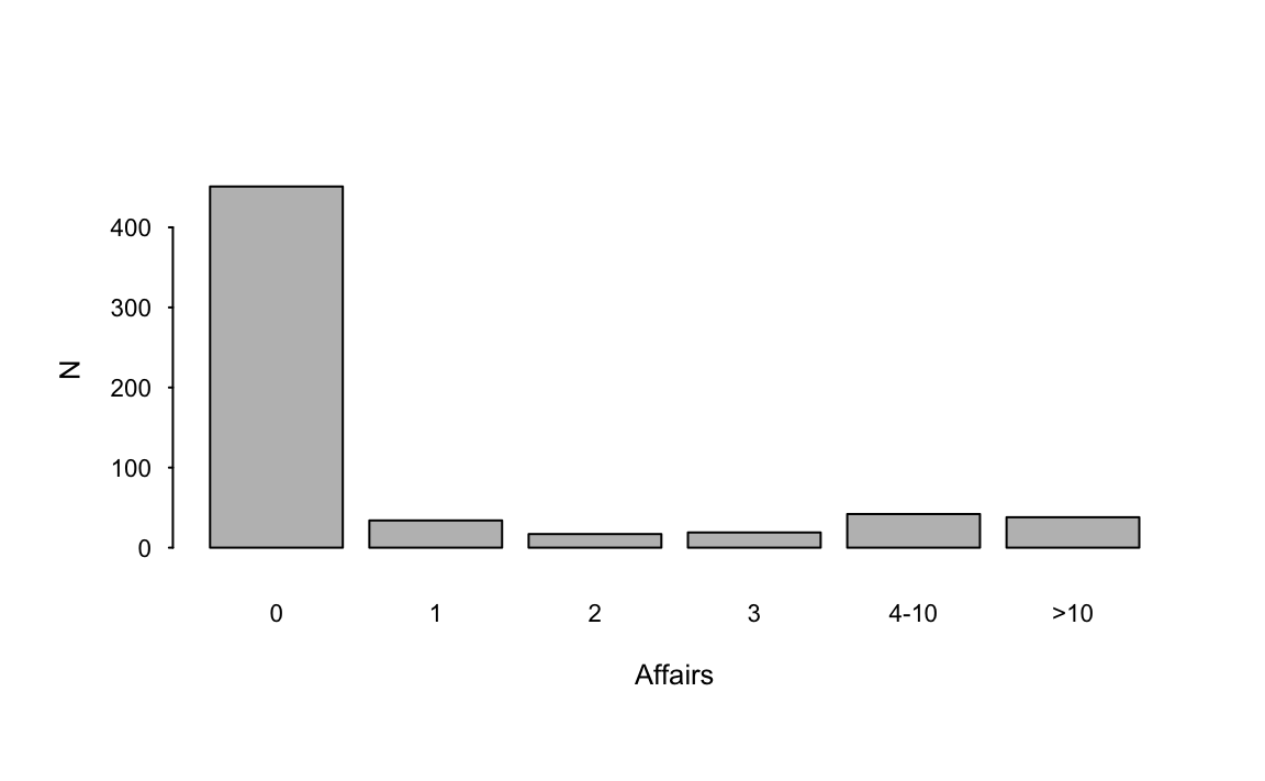
This chapter shows how the framework and tools introduced in Parts I and II help us give meaning to estimates obtained by fitting a categorical or ordinal outcome model.

We say that the outcome variable of a regression model is categorical when it is discrete, involves a finite number of categories, and does not have a natural ordering. Categorical outcomes are very common in data analysis, for example, when one wishes to model the choice of a mode of transportation (e.g., car, bus, bike, walk). A popular way to approach such data is to fit a multinomial logit model.

We say that the outcome variable of a regression model is ordinal when it is discrete, involves a finite number of categories, and has a natural ordering. Ordinal outcomes are very common in data analysis, for example, when one wishes to model levels of satisfaction (e.g., very dissatisfied, dissatisfied, neutral, satisfied, very satisfied). A popular way to approach such data is to fit an ordered probit model. In such a model, the probability of each category \(j\) of the outcome variable is modeled as (Cameron and Trivedi 2005)

\[P(Y = j) = \Phi(\theta_j - \mathbf{X}\beta) - \Phi(\theta_{j-1} - \mathbf{X}\beta)\]

where \(\mathbf{X}\) represents the vector of predictors, \(\beta\) the vector of coefficients, \(\theta_j\) and \(\theta_{j-1}\) the threshold parameters defining the boundaries between categories \(j\) and \(j-1\), and \(\Phi\) the standard normal cumulative distribution function.

The distinguishing feature of models like the multinomial logit or ordered probit is that they estimate different parameters for each level the outcome variable. This allows the analyst to estimate different quantities of interest—predictions, counterfactual comparisons, and slopes—for each level of the dependent variable. This chapter focuses on the ordered probit case, but the same workflow applies to a much wider class of models, including other multinomial and ordered approaches.

Let’s consider the dataset on extramarital affairs, collected in 1969 by the magazine Psychology Today, and analyzed in Fair (1978). These data include 601 survey responses on demographic, marital, and personal characteristics of married Americans: gender, age, years married, children, religiousness, education, occupation, and self-rated happiness in marriage.

The outcome in our analyses is affairs, a variable that records the self-reported frequency of extramarital sexual encounters in the past year: 0, 1, 2, 3, 4-10 or >10. The following code loads the data and plots the distribution of the outcome.

library(MASS)
library(ggplot2)
library(marginaleffects)
dat = get_dataset("affairs")
barplot(table(dat$affairs), ylab = "N", xlab = "Affairs")

Figure 11.1: Distribution of the self-reported number of extra-marital affairs during 12 months preceding the survey (Fair, 1978).

To study the determinants of the number of extramarital affairs, we specify an ordered probit regression model with three predictors: a binary variable indicating whether a survey respondent has children, the number of years since they got married, and a binary indicator for gender. To fit the model, we use the polr() function in the MASS package.

mod = polr(
  affairs ~ children + yearsmarried + gender,
  method = "probit", data = dat, Hess = TRUE)
summary(mod)


Coefficients:
                Value Std. Error t value
childrenyes   0.17290     0.1506  1.1477
yearsmarried  0.03457     0.0116  2.9793
genderwoman  -0.08851     0.1075 -0.8234

Intercepts:
         Value   Std. Error t value
0|1       1.0553  0.1336     7.8970
1|2       1.2524  0.1357     9.2300
2|3       1.3647  0.1372     9.9471
3|4-10    1.5057  0.1394    10.8010
4-10|>10  1.9363  0.1495    12.9536

The coefficients in this model can be viewed as measuring changes in a latent variable, associated to changes in the predictors. Unfortunately, building intuition about this latent variable is complicated, and the parameter estimates do not have a straightforward interpretation. Instead of focusing on those estimates, do what we have done throughout this book, and transform raw parameters into more intuitive quantities of interest: predictions, counterfactual comparisons, and slopes.

11.1 Predictions

The first step of our post-estimation workflow is to compute average predictions. In a categorical outcome model, predictions are expressed on a probability scale. Crucially, the model allows us to make one prediction for every level of the outcome variable.

Imagine that we are specifically interested in the expected number of affairs for a woman with children who has been married for 10 years. To compute this quantity, we use the datagrid() function to build a grid, and call the predictions() function.¹

p = predictions(mod, newdata = datagrid(
  children = "yes",
  yearsmarried = 10,
  gender = "woman"))
p

Group	children	yearsmarried	gender	Estimate	Std. Error	z	Pr(>\|z\|)	2.5 %	97.5 %
0	yes	10	woman	0.7341	0.02755	26.65	<0.001	0.6801	0.7881
1	yes	10	woman	0.0605	0.01041	5.81	<0.001	0.0401	0.0809
2	yes	10	woman	0.0304	0.00746	4.08	<0.001	0.0158	0.0451
3	yes	10	woman	0.0339	0.00795	4.27	<0.001	0.0184	0.0495
4-10	yes	10	woman	0.0750	0.01262	5.94	<0.001	0.0503	0.0998
>10	yes	10	woman	0.0660	0.01310	5.04	<0.001	0.0403	0.0917

This fitted model predicts that there is a 73% probability that this woman will have no extra-marital affair, and a 6% chance that she will have one.

Instead of reporting predicted probabilities for individual cases, we can compute them for all individuals in the dataset, and then average them. As in previous chapters, calling the avg_predictions() returns marginal predictions.

p = avg_predictions(mod)
p

Group	Estimate	Std. Error	z	Pr(>\|z\|)	2.5 %	97.5 %
0	0.7497	0.01739	43.12	<0.001	0.7157	0.7838
1	0.0567	0.00944	6.01	<0.001	0.0382	0.0752
2	0.0285	0.00680	4.19	<0.001	0.0152	0.0418
3	0.0317	0.00715	4.44	<0.001	0.0177	0.0457
4-10	0.0702	0.01039	6.76	<0.001	0.0498	0.0906
>10	0.0631	0.00986	6.40	<0.001	0.0438	0.0824

Since we are working with a categorical outcome model, the avg_predictions() function automatically returns one average predicted probability per outcome level. The group identifiers are available in the group column of the output data frame.

colnames(p)

[1] "group"     "estimate"  "std.error" "statistic" "p.value"   "s.value"  
[7] "conf.low"  "conf.high"

p$group

[1] 0    1    2    3    4-10 >10 
Levels: 0 1 2 3 4-10 >10

Unsurprisingly, given Figure 11.1, the expected probability that affairs=0 is much higher than that of any of the other outcome levels (75%). In contrast, the average predicted probability that survey respondents have over 10 extramarital affairs in a year is 6%.

As we saw in Chapter 5, it is easy to compute average predictions for different subgroups. For instance, if we want to know the expected probability of each outcome level, for survey respondents with and without children, we call the following code.

p <- avg_predictions(mod, by = "children")
head(p, 2)

Group	children	Estimate	Std. Error	z	Pr(>\|z\|)	2.5 %	97.5 %
0	no	0.839	0.0275	30.5	<0.001	0.785	0.893
0	yes	0.714	0.0214	33.5	<0.001	0.672	0.756

On average, the predicted probability that a survey respondent without children has zero affairs is 84%. In contrast, the average predicted probability for a respondent with children is 71%.

We can also plot these figures with an analogous call, using the by argument to marginalize predictions across combinations of outcome group and children predictor.

plot_predictions(mod, by = c("group", "children")) +
  labs(x = "Number of affairs", y = "Average predicted probability")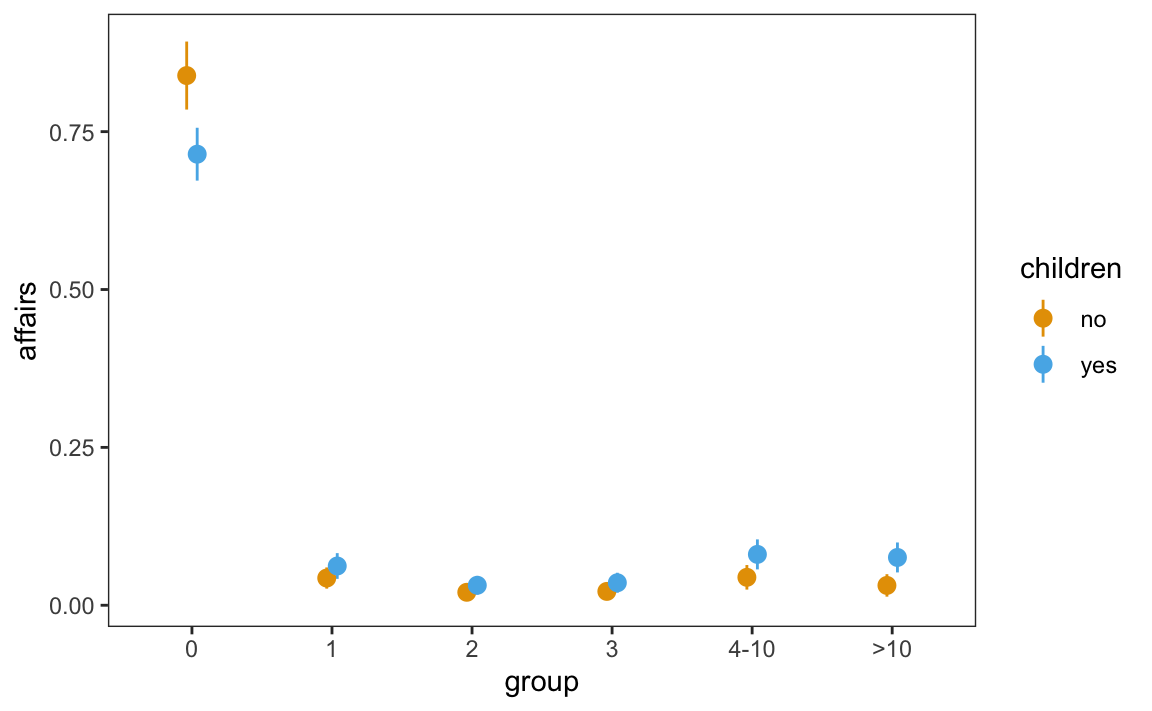

Figure 11.2: Average predicted probabilities for each outcome level, for the subpopulations with and without children.

Figure 11.2 shows again that the most likely survey response, by far, is zero. Moreover, the graph suggests that differences in average predicted probabilities between people with and without children are quite small. This impression will be confirmed in the next section, where we adopt an explicitly counterfactual approach.

In some cases, it can be useful to combine different outcome level categories. For example, the analyst may wish to know what are the chances that survey respondent will report at least one affair. To do this, we must compute the sum of all predicted probabilities for group values above 0.

One powerful strategy is to define a custom function to use in the hypothesis argument of avg_predictions(). As stated in the function manual,² custom hypothesis functions must accept the same data frame that we obtain when calling a function without the hypothesis argument, that is, a data frame with group, term, and estimate columns. The custom function can then process this input and return a new data frame with term and estimate columns.

For example, the custom function defined below accepts a data frame x, collapses the predicted probabilities by group categories, and returns a data frame of new estimates.

hyp = function(x) {
  x$term = ifelse(x$group == "0", "0", ">0")
  aggregate(estimate ~ term + children, FUN = sum, data = x)
}
p = avg_predictions(mod, by = "children", hypothesis = hyp)
p

Term	children	Estimate	Std. Error	z	Pr(>\|z\|)	2.5 %	97.5 %
>0	no	0.161	0.0275	5.87	<0.001	0.107	0.215
0	no	0.839	0.0275	30.53	<0.001	0.785	0.893
>0	yes	0.286	0.0214	13.38	<0.001	0.244	0.328
0	yes	0.714	0.0214	33.45	<0.001	0.672	0.756

On average, the predicted probability that a survey respondent without children will report at least one affair is 84%.

The custom function above applied a sum by subgroup using the aggregate() function, which has been available in base R since the 20th century. The same result can be obtained using the tidyverse idiom.

library(tidyverse)
hyp = function(x) {
  x %>% 
    mutate(term = if_else(group == "0", "0", ">0")) %>%
    summarize(estimate = sum(estimate), .by = c("term", "children"))
}
avg_predictions(mod, by = "children", hypothesis = hyp)

11.2 Counterfactual comparisons

After looking at predictions, it makes sense to adopt an explicitly counterfactual perspective, to quantity the strength of association between predictors and outcome. Our first objective is to answer this question: What would happen to the reported number of affairs if we increased the number of years married, while holding other predictors constant?

To answer this question, we use the avg_comparisons() function, and define the shift in focal predictor using the variables argument.³

avg_comparisons(mod, variables = list(yearsmarried = 5))

Group	Estimate	Std. Error	z	Pr(>\|z\|)	2.5 %	97.5 %
0	-0.05617	0.01940	-2.89	0.00379	-0.094199	-0.01814
1	0.00687	0.00236	2.91	0.00363	0.002241	0.01150
2	0.00427	0.00168	2.54	0.01094	0.000981	0.00756
3	0.00551	0.00215	2.56	0.01040	0.001296	0.00973
4-10	0.01590	0.00580	2.74	0.00607	0.004543	0.02726
>10	0.02362	0.00923	2.56	0.01053	0.005521	0.04171

cmp = avg_comparisons(mod, variables = list(yearsmarried = 5))

On average, increasing the yearsmarried variable by 5 reduces the predicted probability that affairs equals zero by 5.6 percentage points. On average, increasing yearsmarried by 5 increases the predicted probability that affairs is greater than 10 by 2.4 percentage points. These counterfactual comparisons are associated with small \(p\) values, so we can reject the null hypothesis that yearsmarried has no effect on the predicted number of affairs.

In contrast, if we estimate the counterfactual effect of gender, we find that differences in predicted probabilities are small and statistically insignificant. We cannot reject the null hypothesis that gender has no effect on affairs.

avg_comparisons(mod, variables = "gender")

Group	Estimate	Std. Error	z	Pr(>\|z\|)	2.5 %	97.5 %
0	0.02736	0.03324	0.823	0.411	-0.03779	0.09251
1	-0.00373	0.00458	-0.815	0.415	-0.01271	0.00524
2	-0.00225	0.00278	-0.808	0.419	-0.00769	0.00320
3	-0.00284	0.00350	-0.811	0.417	-0.00970	0.00402
4-10	-0.00786	0.00959	-0.819	0.413	-0.02666	0.01095
>10	-0.01068	0.01305	-0.818	0.413	-0.03626	0.01491

In conclusion, this chapter has demonstrated how categorical and ordinal outcome models, such as the ordered probit model, can be effectively used to interpret complex data. By transforming raw parameter estimates into intuitive quantities like predictions and counterfactual comparisons, analysts can gain meaningful insights into the data. This approach not only enhances the interpretability of the model results but also facilitates clearer communication of findings to a broader audience.

Chapter 5 ↩︎
In R, you can access the function manual by typing ?avg_predictions. In Python, it can be accessed by typing help(avg_predictions). The manual is also hosted at https://marginaleffects.com ↩︎
Section 6.2.1 ↩︎