library(marginaleffects)
dat = get_dataset("thornton")
mod = lm(outcome ~ incentive, data = dat)
coef(mod)
(Intercept) incentive
0.3397746 0.4510603 The analysis of experiments is a common use case for the marginaleffects package, which provides researchers with a powerful toolkit for estimating treatment effects, interpreting interactions, and visualizing results across experimental conditions. To illustrate these benefits, this chapter discusses two common applications: covariate adjustment, and the interpretation of results from a 2-by-2 factorial experiment. The marginaleffects.com website hosts more tutorials to guide the analysis and interpretation of a variety of other experimental designs.
The first application that we consider is a simple two-arm experiment, where participants are randomly assigned to a treatment or a control group. Our goal is to estimate the average treatment effect, while adjusting for covariates. As in previous chapters, we use data from Thornton (2008). The outcome is a binary variable that records if individuals traveled to the clinic to learn their HIV status. The treatment is a financial incentive, randomly given to participants, with the goal of encouraging testing.
Since the incentive treatment was randomized, we can estimate the average treatment effect (ATE) easily via linear regression on the binary outcome. This is the so-called “linear probability model” (LPM).
library(marginaleffects)
dat = get_dataset("thornton")
mod = lm(outcome ~ incentive, data = dat)
coef(mod)(Intercept) incentive
0.3397746 0.4510603 import polars as pl
from marginaleffects import *
from statsmodels.formula.api import logit, ols
dat = get_dataset("thornton")
mod = ols("outcome ~ incentive", data = dat.to_pandas()).fit()
mod.paramsIntercept 0.339775
incentive 0.451060
dtype: float64As demonstrated in previous chapters, the marginaleffects package implements post-estimation transformations that are essentially agnostic with respect to the choice of model. Hence, the workflow described below would remain unchanged if the analyst chose to fit a GLM (or other) model instead of this LPM.
The coefficient associated to the incentive variable shows the difference in the predicted probability of seeking one’s test result, between those who received the incentive and those who did not. This result is identical to what we would obtain via G-computation, using the avg_comparisons() function.1 One benefit of using this function instead of looking at individual coefficients, is that the vcov argument allows us to easily report heteroskedasticity-consistent, robust, or clustered standard errors.2
avg_comparisons(mod, variables = "incentive", vcov = "HC2")| Estimate | Std. Error | z | Pr(>|z|) | 2.5 % | 97.5 % |
|---|---|---|---|---|---|
| 0.451 | 0.0209 | 21.6 | <0.001 | 0.41 | 0.492 |
avg_comparisons(mod, variables = "incentive", vcov = "HC2")shape: (1, 7)
┌──────────┬───────────┬──────┬─────────┬─────┬──────┬───────┐
│ Estimate ┆ Std.Error ┆ z ┆ P(>|z|) ┆ S ┆ 2.5% ┆ 97.5% │
│ --- ┆ --- ┆ --- ┆ --- ┆ --- ┆ --- ┆ --- │
│ str ┆ str ┆ str ┆ str ┆ str ┆ str ┆ str │
╞══════════╪═══════════╪══════╪═════════╪═════╪══════╪═══════╡
│ 0.451 ┆ 0.0209 ┆ 21.6 ┆ 0 ┆ inf ┆ 0.41 ┆ 0.492 │
└──────────┴───────────┴──────┴─────────┴─────┴──────┴───────┘
Term: incentive
Contrast: 1 - 0When the treatment is randomized, it is not strictly necessary to adjust for covariates in order to obtain an unbiased estimate of the average treatment effect. However, including control variables in the regression model can improve the precision of estimates, by reducing the unexplained variance in the outcome. This is an attractive strategy, but it must be applied with care. Indeed, as Freedman (2008) points out, naively inserting control variables in additive fashion to our model equation has an important downside: it can introduce small-sample bias and degrade asymptotic precision. To avoid this problem, Lin (2013) recommends a simple solution: interacting all covariates with the treatment indicator, and reporting heteroskedasticity-robust standard errors.
mod = lm(outcome ~ incentive * (age + distance + hiv2004), data = dat)mod = ols("outcome ~ incentive * (age + distance + hiv2004)",
data=dat.to_pandas()).fit()Interpreting the results of this model is not straightforward, since there are multiple coefficients, with several multiplicative interactions.3
coef(mod) (Intercept) incentive age distance
0.309537645 0.496482649 0.003495124 -0.042323583
hiv2004 incentive:age incentive:distance incentive:hiv2004
0.013562711 -0.002177778 0.014571883 -0.070766068 mod.paramsIntercept 0.309538
incentive 0.496483
age 0.003495
distance -0.042324
hiv2004 0.013563
incentive:age -0.002178
incentive:distance 0.014572
incentive:hiv2004 -0.070766
dtype: float64Thankfully, we can simply call avg_comparisons() again to get the covariate-adjusted estimate, along with robust standard errors.
avg_comparisons(mod,
variables = "incentive",
vcov = "HC2")| Estimate | Std. Error | z | Pr(>|z|) | 2.5 % | 97.5 % |
|---|---|---|---|---|---|
| 0.449 | 0.0209 | 21.5 | <0.001 | 0.408 | 0.49 |
avg_comparisons(mod, variables = "incentive", vcov = "HC2")shape: (1, 7)
┌──────────┬───────────┬──────┬─────────┬─────┬───────┬───────┐
│ Estimate ┆ Std.Error ┆ z ┆ P(>|z|) ┆ S ┆ 2.5% ┆ 97.5% │
│ --- ┆ --- ┆ --- ┆ --- ┆ --- ┆ --- ┆ --- │
│ str ┆ str ┆ str ┆ str ┆ str ┆ str ┆ str │
╞══════════╪═══════════╪══════╪═════════╪═════╪═══════╪═══════╡
│ 0.449 ┆ 0.0209 ┆ 21.5 ┆ 0 ┆ inf ┆ 0.408 ┆ 0.49 │
└──────────┴───────────┴──────┴─────────┴─────┴───────┴───────┘
Term: incentive
Contrast: 1 - 0This suggests that, on average, receiving a monetary incentive increases by 44.9 percentage points the probability of seeking one’s HIV test result.
A factorial experiment is a type of study design that allows researchers to assess the effects of two or more randomized treatments simultaneously, with each treatment having multiple levels or conditions. A common example is the 2-by-2 design, where two variables with two levels are randomized simultaneously and independently. This setup enables the evaluator to quantify the effects of each treatment, but also to examine if the treatments interact with one another.
In medicine, factorial experiments are widely used to explore complex phenomena like drug interactions, where researchers test different combinations of treatments to see how they affect patient outcomes. In plant physiology, they could be used to see how combinations of temperature and humidity affect photosynthesis. In a business context, a company could use a factorial design to test if different advertising strategies and price points drive sales.
To illustrate, let’s consider a simple data set with 32 observations, a numeric outcome \(Y\), and two treatments with two levels: \(T_a=\{0,1\}\) and \(T_b=\{0,1\}\). We fit a linear regression model with each treatment entered individually, along with their multiplicative interaction.4
library(marginaleffects)
dat = get_dataset("factorial_01")
mod = lm(Y ~ Ta + Tb + Ta:Tb, data = dat)
coef(mod)
(Intercept) Ta Tb Ta:Tb
15.050000 5.692857 4.700000 2.928571 dat = get_dataset("factorial_01")
mod = ols("Y ~ Ta + Tb + Ta:Tb", data = dat.to_pandas()).fit()
mod.paramsIntercept 15.050000
Ta 5.692857
Tb 4.700000
Ta:Tb 2.928571
dtype: float64We can plot the model’s predictions for each combination of \(T_a\) and \(T_b\) using the plot_predictions function.
plot_predictions(mod, by = c("Ta", "Tb"))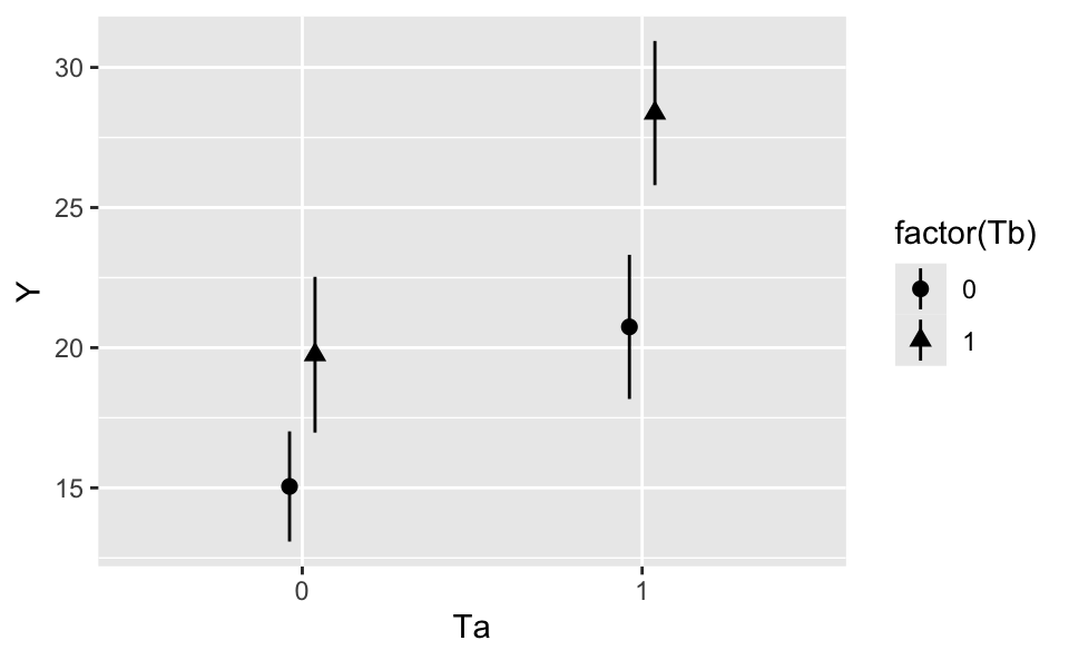
plot_predictions(mod, by = ["Ta", "Tb"]).show()
Now, imagine we want to estimate the effect of changing \(T_a\) from 0 to 1 on \(Y\), while holding \(T_b=0\). We define two counterfactual values of \(Y\) and take their difference.
\[\begin{align*} \hat{Y} &= \hat{\beta}_1 + \hat{\beta}_2 \cdot T_a + \hat{\beta}_3 \cdot T_b + \hat{\beta}_4 \cdot T_a \cdot T_b\\ \hat{Y}_{T_a=0,T_b=0} &= \hat{\beta}_1 + \hat{\beta}_2 \cdot 0 + \hat{\beta}_3 \cdot 0 + \hat{\beta}_4 \cdot 0 \cdot 0\\ \hat{Y}_{T_a=1,T_b=0} &= \hat{\beta}_1 + \hat{\beta}_2 \cdot 1 + \hat{\beta}_3 \cdot 0 + \hat{\beta}_4 \cdot 1 \cdot 0\\ \hat{Y}_{T_a=1,T_b=0} - \hat{Y}_{T_a=0,T_b=0} &= \hat{\beta}_2 = 5.693 \end{align*}\]
We can use a similar approach to estimate a cross-contrast, that is, the effect of changing both \(T_a\) and \(T_b\) from 0 to 1 simultaneously.
\[\begin{align*} \hat{Y}_{T_a=0,T_b=0} &= \hat{\beta}_1 + \hat{\beta}_2 \cdot 0 + \hat{\beta}_3 \cdot 0 + \hat{\beta}_4 \cdot 0 \cdot 0\\ \hat{Y}_{T_a=1,T_b=1} &= \hat{\beta}_1 + \hat{\beta}_2 \cdot 1 + \hat{\beta}_3 \cdot 1 + \hat{\beta}_4 \cdot 1 \cdot 1\\ \hat{Y}_{T_a=1,T_b=1} - \hat{Y}_{T_0=1,T_b=0} &= \hat{\beta}_2 + \hat{\beta}_3 + \hat{\beta}_4 = 13.321 \end{align*}\]
In a simple 2-by-2 experiment, this arithmetic is fairly simple. However, things can quickly get complicated when more treatment conditions are introduced, or when regression models include non-linear components. Moreover, even if we can take sums of coefficients to get the estimates we care about, computing standard errors (classical or robust) is non-trivial. Thus, it is convenient to use software like marginaleffects to do the hard work for us.
To estimate the effect of \(T_a\) on \(Y\), holding \(T_b=0\) constant, we use the avg_comparisons() function. The variables argument specifies the treatment of interest, and the newdata argument specifies the levels of the other treatment(s) at which we want to evaluate the contrast. In this case, we use newdata=subset(Tb == 0) to compute the quantity of interest only in the subset of observations where \(T_b=0\).
avg_comparisons(mod,
  variables = "Ta",
newdata = subset(Tb == 0))| Estimate | Std. Error | z | Pr(>|z|) | 2.5 % | 97.5 % |
|---|---|---|---|---|---|
| 5.69 | 1.65 | 3.45 | <0.001 | 2.46 | 8.93 |
avg_comparisons(mod, variables = "Ta",
  newdata = dat.filter(pl.col("Tb") == 0))
shape: (1, 7)
┌──────────┬───────────┬──────┬─────────┬──────┬──────┬───────┐
│ Estimate ┆ Std.Error ┆ z ┆ P(>|z|) ┆ S ┆ 2.5% ┆ 97.5% │
│ --- ┆ --- ┆ --- ┆ --- ┆ --- ┆ --- ┆ --- │
│ str ┆ str ┆ str ┆ str ┆ str ┆ str ┆ str │
╞══════════╪═══════════╪══════╪═════════╪══════╪══════╪═══════╡
│ 5.69 ┆ 1.65 ┆ 3.45 ┆ 0.0018 ┆ 9.11 ┆ 2.31 ┆ 9.08 │
└──────────┴───────────┴──────┴─────────┴──────┴──────┴───────┘
Term: Ta
Contrast: 1 - 0To estimate a cross-contrast, we specify each treatment of interest in the variables argument, and set cross=TRUE. This gives the estimated effect of simultaneously moving \(T_a\) and \(T_b\) from 0 to 1.
avg_comparisons(mod,
  variables = c("Ta", "Tb"),
cross = TRUE)| C: Ta | C: Tb | Estimate | Std. Error | z | Pr(>|z|) | 2.5 % | 97.5 % |
|---|---|---|---|---|---|---|---|
| 1 - 0 | 1 - 0 | 13.3 | 1.65 | 8.07 | <0.001 | 10.1 | 16.6 |
avg_comparisons(mod, variables=["Ta", "Tb"], cross=True)shape: (1, 9)
┌───────┬───────┬──────────┬───────────┬───┬──────────┬──────┬──────┬───────┐
│ C: Ta ┆ C: Tb ┆ Estimate ┆ Std.Error ┆ … ┆ P(>|z|) ┆ S ┆ 2.5% ┆ 97.5% │
│ --- ┆ --- ┆ --- ┆ --- ┆ ┆ --- ┆ --- ┆ --- ┆ --- │
│ str ┆ str ┆ str ┆ str ┆ ┆ str ┆ str ┆ str ┆ str │
╞═══════╪═══════╪══════════╪═══════════╪═══╪══════════╪══════╪══════╪═══════╡
│ 1 - 0 ┆ 1 - 0 ┆ 13.3 ┆ 1.65 ┆ … ┆ 8.74e-09 ┆ 26.8 ┆ 9.94 ┆ 16.7 │
└───────┴───────┴──────────┴───────────┴───┴──────────┴──────┴──────┴───────┘
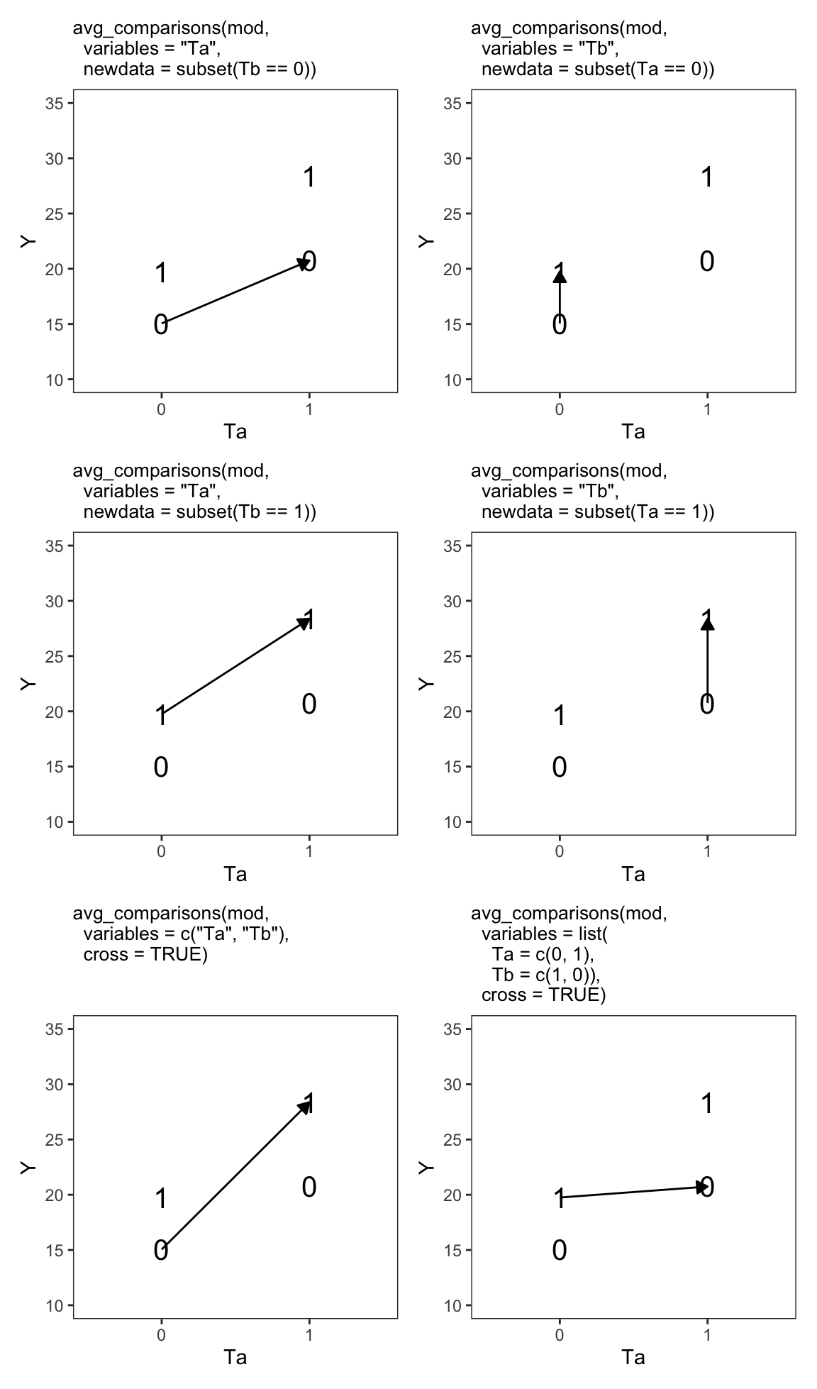
Term: crossFigure 9.1 shows six contrasts of interest in a 2-by-2 experimental design. The vertical axis shows the value of the outcome variable in each treatment group. The horizontal axis shows the value of the first treatment \(T_a\). The shape of points—0 or 1—represents the value of the \(T_b\) treatment. For example, the “1” symbol in the top left shows the average value of \(Y\) in the \(T_a=0,T_b=1\) group.
In each panel, the arrow links two treatment groups that we want to compare. For example, in the top-left panel we compare \(\hat{Y}_{T_a=0,T_b=0}\) to \(\hat{Y}_{T_a=1,T_b=0}\). In the bottom-right panel, we compare \(\hat{Y}_{T_a=0,T_b=1}\) to \(\hat{Y}_{T_a=1,T_b=0}\). The avg_comparisons() call at the top of each panel shows how to use marginaleffects to compute the difference in \(Y\) that results from the illustrated change in treatment conditions.
One reason factorial experiments are so popular is that they allow researchers to assess the possibility that treatments interact with one another. Indeed, in some cases, the effect of a treatment \(T_a\) will be stronger (or weaker) at different values of treatment \(T_b\).
To check this, let us estimate the effect of a change from 0 to 1 in \(T_a\), in the subsets of observations with different values of \(T_b\).
cmp <- avg_comparisons(mod, variables = "Ta", by = "Tb")
cmp| Tb | Estimate | Std. Error | z | Pr(>|z|) | 2.5 % | 97.5 % |
|---|---|---|---|---|---|---|
| 0 | 5.69 | 1.65 | 3.45 | <0.001 | 2.46 | 8.93 |
| 1 | 8.62 | 1.93 | 4.46 | <0.001 | 4.84 | 12.41 |
avg_comparisons(mod, variables = "Ta", by = "Tb")shape: (2, 8)
┌─────┬──────────┬───────────┬──────┬─────────┬──────┬──────┬───────┐
│ Tb ┆ Estimate ┆ Std.Error ┆ z ┆ P(>|z|) ┆ S ┆ 2.5% ┆ 97.5% │
│ --- ┆ --- ┆ --- ┆ --- ┆ --- ┆ --- ┆ --- ┆ --- │
│ str ┆ str ┆ str ┆ str ┆ str ┆ str ┆ str ┆ str │
╞═════╪══════════╪═══════════╪══════╪═════════╪══════╪══════╪═══════╡
│ 0 ┆ 5.69 ┆ 1.65 ┆ 3.45 ┆ 0.0018 ┆ 9.11 ┆ 2.31 ┆ 9.08 │
│ 1 ┆ 8.62 ┆ 1.93 ┆ 4.46 ┆ 0.00012 ┆ 13 ┆ 4.66 ┆ 12.6 │
└─────┴──────────┴───────────┴──────┴─────────┴──────┴──────┴───────┘
Term: Ta
Contrast: 1 - 0The estimated effect of \(T_a\) on \(Y\) is equal to 5.69 when \(T_b=0\), but equal to 8.62 when \(T_b=1\). At first glance, it thus seems that the effect of \(T_a\) is stronger when \(T_b=1\).
Is the difference between estimated treatment effects statistically significant? Does \(T_b\) moderate the effect the effect of \(T_a\)? Is there treatment heterogeneity or interaction between \(T_a\) and \(T_b\)? To answer these questions, we use the hypothesis argument and check if the difference between subgroup estimates is significant.
avg_comparisons(mod,
  variables = "Ta",
  by = "Tb",
hypothesis = "b2 - b1 = 0")| Hypothesis | Estimate | Std. Error | z | Pr(>|z|) | 2.5 % | 97.5 % |
|---|---|---|---|---|---|---|
| b2-b1=0 | 2.93 | 2.54 | 1.15 | 0.249 | -2.05 | 7.91 |
avg_comparisons(mod, variables = "Ta", by = "Tb",
  hypothesis = "b1 - b0 = 0")
shape: (1, 7)
┌──────────┬───────────┬──────┬─────────┬──────┬───────┬───────┐
│ Estimate ┆ Std.Error ┆ z ┆ P(>|z|) ┆ S ┆ 2.5% ┆ 97.5% │
│ --- ┆ --- ┆ --- ┆ --- ┆ --- ┆ --- ┆ --- │
│ str ┆ str ┆ str ┆ str ┆ str ┆ str ┆ str │
╞══════════╪═══════════╪══════╪═════════╪══════╪═══════╪═══════╡
│ 2.93 ┆ 2.54 ┆ 1.15 ┆ 0.259 ┆ 1.95 ┆ -2.28 ┆ 8.13 │
└──────────┴───────────┴──────┴─────────┴──────┴───────┴───────┘
Term: b1-b0=0While there is a difference between our two estimates, the \(z\) statistic and \(p\) value indicate that this difference is not statistically significant. Therefore, we cannot reject the null hypothesis that the effect of \(T_a\) is the same, regardless of the value of \(T_b\).
Lin (2013) recommends interacting the treatment indicator with de-meaned control variables. By doing so, the linear regression coefficient of the treatment variable become directly interpretable. Using the avg_comparisons() function is more convenient, because it produces the same results without forcing us to de-mean control variables first. As Lin notes, it may still be a good idea to report the unadjusted estimate, for transparency reasons, and to avoid the temptation of specific-searching.↩︎