17  Interrupted Times Series

Interrupted Time Series (ITS) analysis is a widely used research design that aims to infer the impact of a discrete intervention or event by examining changes in an outcome measure over time. It finds applications in various fields, including public health policies—such as evaluating the effect of vaccination campaigns—and educational settings—like assessing curriculum reform. The key motivation behind ITS is to leverage data already being collected, identify a clear “interruption” at a known point in time (e.g., when a policy was enacted), and then compare the behavior of the outcome measure before and after this interruption.

Although ITS can be extremely useful, it also poses substantial methodological and practical challenges. Unlike experimental or quasi-experimental approaches, ITS relies on very strong assumptions about the continuity or predictability of the outcome’s pre-intervention trajectory. Unobserved confounding events and gradual policy rollouts can violate these assumptions, complicating efforts to attribute changes solely to the interruption.

ITS shares some similarities with the popular difference-in-differences (DiD) approach, in which outcomes in a treated group are contrasted with those in an untreated comparison group. Meeting the assumptions required for credible inference with DiD is extremely challenging, as is attested by recent methodological developments in this field (Roth et al. 2023). ITS is arguably even more difficult to get right, since it typically relies only on a single times series, and thus lacks a true control group.

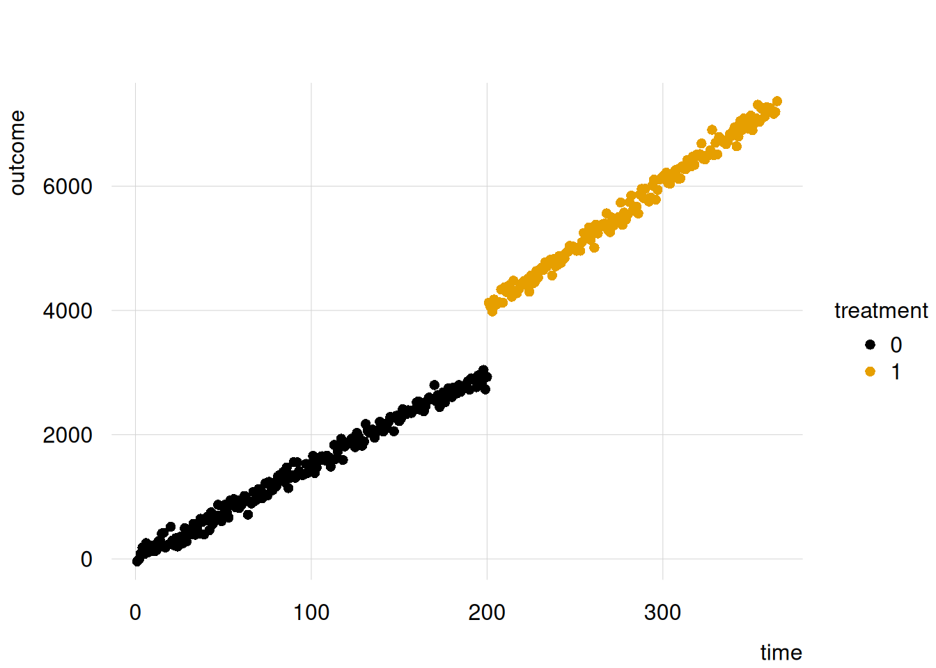
This article shows how to use the marginaleffects package to analyze a simple ITS setup. To illustrate, we consider a dataset simulated by this code:

R

library(marginaleffects)
library(tinyplot)
tinytheme("ipsum")
set.seed(48103)

# number of days
n <- 365

# intervention at day
intervention <- 200

# time index from 1 to 365
time <- c(1:n)

# treatment variable: 0 before the intervention and 1 after
treatment <- c(rep(0, intervention), rep(1, n - intervention))

# outcome equation
outcome <- 
  10 +  # pre-intervention intercept
  15 * time +  # pre-intervention slope (trend)
  20 * treatment +  # post-intervention intercept (shift of 10)
  5 * treatment * time + # steeper slope after the intervention
  rnorm(n, mean = 0, sd = 100) # noise

dat <- data.frame(outcome, time, treatment)

Python

import numpy as np
import pandas as pd
import statsmodels.formula.api as smf
from marginaleffects import avg_slopes, comparisons, predictions
from plotnine import (
    aes,
    facet_wrap,
    geom_line,
    geom_point,
    ggplot,
    labs,
    scale_color_manual,
    theme_minimal,
)

dat = r.dat.copy()
dat["time"] = dat["time"].astype(int)
dat["treatment"] = dat["treatment"].astype(int)
n = int(r.n)
intervention = int(r.intervention)

The data look like this:

R

library(tinyplot)
tinyplot(outcome ~ time | treatment, type = "p", palette = "okabeito",
    data = transform(dat, treatment = factor(treatment)))

Python

import pandas as pd
from plotnine import aes, geom_point, ggplot, labs, scale_color_manual, theme_minimal

dat = r.dat.copy()
dat["time"] = dat["time"].astype(int)
dat["treatment"] = dat["treatment"].astype(int)
dat_plot = dat.copy()
dat_plot["treatment"] = dat_plot["treatment"].astype(str)

okabe_ito = [
    "#E69F00", "#56B4E9", "#009E73",
    "#F0E442", "#0072B2", "#D55E00",
    "#CC79A7", "#999999"
]

plot = (
    ggplot(dat_plot, aes(x="time", y="outcome", color="treatment"))
    + geom_point()
    + scale_color_manual(values=okabe_ito[:2])
    + theme_minimal()
    + labs(x="Time", y="Outcome", color="treatment")
)
plot.show()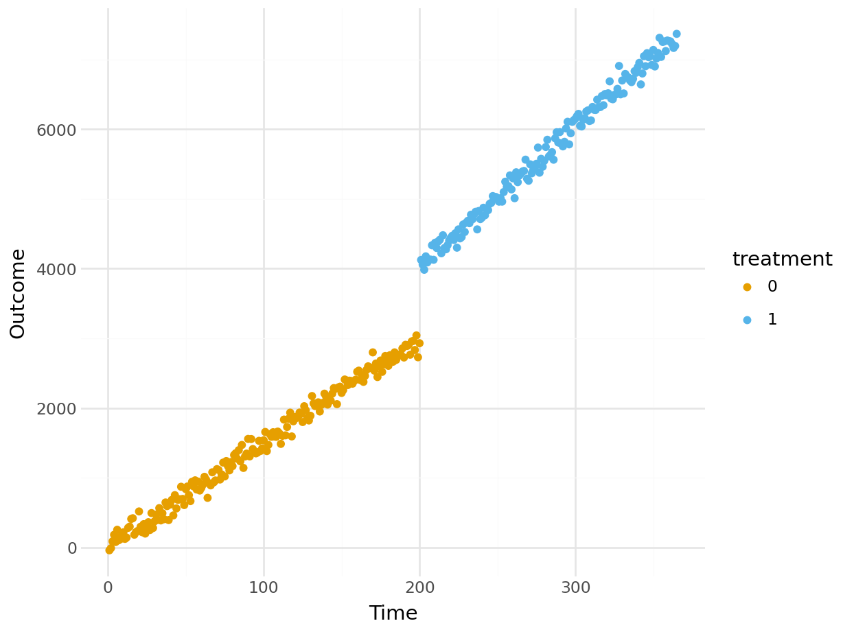

Often, analysts will model such data using a linear regression model with multiplicative interaction, and a specially constructured “time since intervention” variable:

\[ \text{Outcome} = \beta_0 + \beta_1 \text{Time} + \beta_2 \text{Treatment} + \beta_3 \text{Time since intervention} + \varepsilon \]

With marginaleffects, we do not even need to construct this special variable.¹ All we have to do is fit this mathematically equivalent—and simpler—model:

\[ \text{Outcome} = \alpha_0 + \alpha_1 \text{Time} + \alpha_2 \text{Treatment} + \alpha_3 \text{Time} \times \text{Treatment} + \varepsilon \]

R

mod <- lm(outcome ~ time * treatment, data = dat)
summary(mod)

Call:
lm(formula = outcome ~ time * treatment, data = dat)

Residuals:
     Min       1Q   Median       3Q      Max 
-261.551  -69.865    0.908   66.543  308.257 

Coefficients:
               Estimate Std. Error t value Pr(>|t|)    
(Intercept)      4.4518    13.6298   0.327    0.744    
time            15.0023     0.1176 127.574   <2e-16 ***
treatment      -17.6430    47.0542  -0.375    0.708    
time:treatment   5.1581     0.1961  26.303   <2e-16 ***
---
Signif. codes:  0 '***' 0.001 '**' 0.01 '*' 0.05 '.' 0.1 ' ' 1

Residual standard error: 96.02 on 361 degrees of freedom
Multiple R-squared:  0.9982,    Adjusted R-squared:  0.9982 
F-statistic: 6.804e+04 on 3 and 361 DF,  p-value: < 2.2e-16

Python

import statsmodels.formula.api as smf

dat = r.dat.copy()
dat["time"] = dat["time"].astype(int)
dat["treatment"] = dat["treatment"].astype(int)
mod_py = smf.ols("outcome ~ time * treatment", data=dat).fit()
print(mod_py.summary())

                            OLS Regression Results                            
==============================================================================
Dep. Variable:                outcome   R-squared:                       0.998
Model:                            OLS   Adj. R-squared:                  0.998
Method:                 Least Squares   F-statistic:                 6.804e+04
Date:                Mon, 01 Jun 2026   Prob (F-statistic):               0.00
Time:                        00:00:38   Log-Likelihood:                -2182.0
No. Observations:                 365   AIC:                             4372.
Df Residuals:                     361   BIC:                             4388.
Df Model:                           3                                         
Covariance Type:            nonrobust                                         
==================================================================================
                     coef    std err          t      P>|t|      [0.025      0.975]
----------------------------------------------------------------------------------
Intercept          4.4518     13.630      0.327      0.744     -22.352      31.256
time              15.0023      0.118    127.574      0.000      14.771      15.234
treatment        -17.6430     47.054     -0.375      0.708    -110.178      74.892
time:treatment     5.1581      0.196     26.303      0.000       4.772       5.544
==============================================================================
Omnibus:                        0.403   Durbin-Watson:                   2.150
Prob(Omnibus):                  0.818   Jarque-Bera (JB):                0.528
Skew:                          -0.005   Prob(JB):                        0.768
Kurtosis:                       2.814   Cond. No.                     2.63e+03
==============================================================================

Notes:
[1] Standard Errors assume that the covariance matrix of the errors is correctly specified.
[2] The condition number is large, 2.63e+03. This might indicate that there are
strong multicollinearity or other numerical problems.

Then, we can use the marginaleffects package to answer a series of scientific questions. For example, what would be the predicted outcome at time 200 with or without intervention?

R

p0 <- predictions(mod, newdata = datagrid(time = 199, treatment = 0))
p1 <- predictions(mod, newdata = datagrid(time = 200, treatment = 1))

p0

 time treatment Estimate Std. Error   z Pr(>|z|)   S 2.5 % 97.5 %
  199         0     2990       13.4 223   <0.001 Inf  2964   3016

Type: response

p1

 time treatment Estimate Std. Error   z Pr(>|z|)   S 2.5 % 97.5 %
  200         1     4019         15 268   <0.001 Inf  3989   4048

Type: response

Python

import pandas as pd
import statsmodels.formula.api as smf
from marginaleffects import predictions

dat = r.dat.copy()
dat["time"] = dat["time"].astype(int)
dat["treatment"] = dat["treatment"].astype(int)
mod_py = smf.ols("outcome ~ time * treatment", data=dat).fit()

p0_py = predictions(
    mod_py,
    newdata=pd.DataFrame({"time": [199], "treatment": [0]}),
    vcov=False
)
p1_py = predictions(
    mod_py,
    newdata=pd.DataFrame({"time": [200], "treatment": [1]}),
    vcov=False
)

print(p0_py)

shape: (1, 1)
┌──────────┐
│ Estimate │
│ ---      │
│ str      │
╞══════════╡
│ 2.99e+03 │
└──────────┘

print(p1_py)

shape: (1, 1)
┌──────────┐
│ Estimate │
│ ---      │
│ str      │
╞══════════╡
│ 4.02e+03 │
└──────────┘

This suggests that the intervention would have increased the outcome by about 1028.9766399 units at time 200. Is the difference between those predictions statistically significant?

R

comparisons(mod, variables = "treatment", newdata = datagrid(time = 200))

 time Estimate Std. Error    z Pr(>|z|)   S 2.5 % 97.5 %
  200     1014       20.2 50.2   <0.001 Inf   974   1054

Term: treatment
Type: response
Comparison: 1 - 0

Python

import pandas as pd
import statsmodels.formula.api as smf
from marginaleffects import comparisons

dat = r.dat.copy()
dat["time"] = dat["time"].astype(int)
dat["treatment"] = dat["treatment"].astype(int)
mod_py = smf.ols("outcome ~ time * treatment", data=dat).fit()

comparisons(
    mod_py,
    variables="treatment",
    newdata=pd.DataFrame({"time": [200], "treatment": [0]}),
    vcov=False
)

shape: (1, 1)
┌──────────┐
│ Estimate │
│ ---      │
│ str      │
╞══════════╡
│ 1.01e+03 │
└──────────┘
Term: treatment
Contrast: 1 - 0

What is the average slope of the outcome equation with respect to time, before and after the intervention?

R

avg_slopes(mod, variables = "time", by = "treatment")

 treatment Estimate Std. Error   z Pr(>|z|)   S 2.5 % 97.5 %
         0     15.0      0.118 128   <0.001 Inf  14.8   15.2
         1     20.2      0.157 128   <0.001 Inf  19.9   20.5

Term: time
Type: response
Comparison: dY/dX

Python

import statsmodels.formula.api as smf
from marginaleffects import avg_slopes

dat = r.dat.copy()
dat["time"] = dat["time"].astype(int)
dat["treatment"] = dat["treatment"].astype(int)
mod_py = smf.ols("outcome ~ time * treatment", data=dat).fit()

avg_slopes(
    mod_py,
    variables="time",
    by="treatment",
    eps=0.01,
    vcov=False
)

shape: (2, 2)
┌───────────┬──────────┐
│ treatment ┆ Estimate │
│ ---       ┆ ---      │
│ str       ┆ str      │
╞═══════════╪══════════╡
│ 0         ┆ 15       │
│ 1         ┆ 20.2     │
└───────────┴──────────┘
Term: time
Contrast: dY/dX

This shows that the outcome increases more rapidly after the intervention.

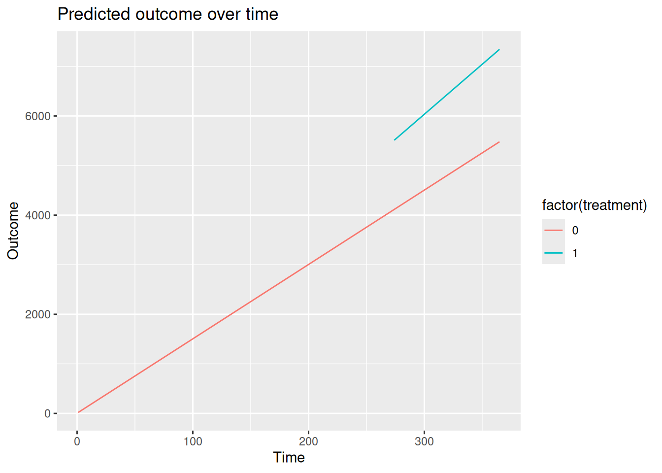
Many analysts like to visualize the results of an ITS analysis, by plotting the predicted outcome for the control group, knowing that these predictions are counterfactual after the intervention. This can be done by first make predictions for all combinations of time and treatment, dropping the observations we do not want to plot, and feeding the data to a plotting package like ggplot2.

R

library(ggplot2)
p <- predictions(mod, variables = c("time", "treatment"))
p <- subset(p, time > intervention | treatment == 0)
ggplot(p, aes(x = time, y = estimate, color = factor(treatment))) +
  geom_line() +
  labs(title = "Predicted outcome over time",
       x = "Time",
       y = "Outcome")

Python

import numpy as np
import pandas as pd
import statsmodels.formula.api as smf
from marginaleffects import predictions
from plotnine import aes, geom_line, ggplot, labs

dat = r.dat.copy()
dat["time"] = dat["time"].astype(int)
dat["treatment"] = dat["treatment"].astype(int)
intervention = int(r.intervention)
mod_py = smf.ols("outcome ~ time * treatment", data=dat).fit()

time_vals = np.sort(dat["time"].unique())
grid = pd.DataFrame(
    [(t, tr) for tr in [0, 1] for t in time_vals],
    columns=["time", "treatment"]
)

p_py = predictions(mod_py, newdata=grid, vcov=False).to_pandas()
p_py = p_py[
    (p_py["time"] > intervention) |
    (p_py["treatment"] == 0)
].copy()
p_py["treatment"] = p_py["treatment"].astype(str)

plot = (
    ggplot(p_py, aes(x="time", y="estimate", color="treatment"))
    + geom_line()
    + labs(title="Predicted outcome over time", x="Time", y="Outcome")
)
plot.show()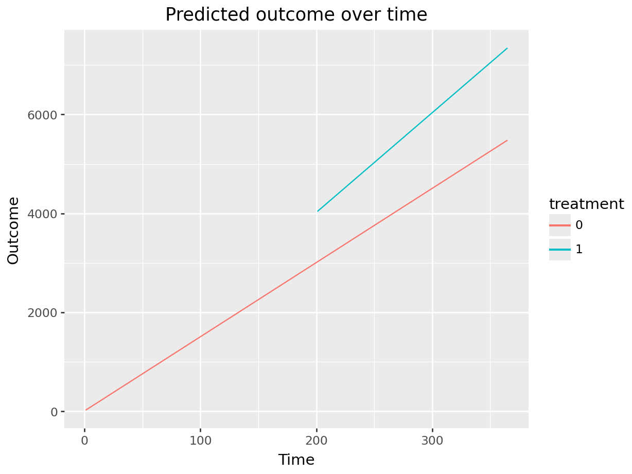

Roth, Jonathan, Pedro H. C. Sant’Anna, Alyssa Bilinski, and John Poe. 2023. “What’s Trending in Difference-in-Differences? A Synthesis of the Recent Econometrics Literature.” Journal of Econometrics 235 (2): 2218–44. https://doi.org/https://doi.org/10.1016/j.jeconom.2023.03.008.

---

1. In fact, analysts should not construct this special variable. The problem is that the time and time_since variables are related, but when we hard-code them, R does not know the mathematical relationship between them.